easing

Code Poetry: Easing Tutorial & Optimizations

Table of Contents

• Overview
• Demos
• Reference
  • Easing Cheat Sheet
  • Comparision of easing functions
  • TL:DR; “Shut up and show me the code!”
• Easing … what is it and why is it important?
  • Parameter t or p
  • Simultaneous Animations
  • Why Javascript?
  • The Color Axis
  • Linear Interpolation: Lerp
  • Non-Linear Interpolation: Slerp
  • Non-linear interpolation: smoothstep
• De Facto Easing Functions
• Easing Cleanup
  • Cleanup - Linear
  • “I’m here for an argument”
  • “Warp Speed, Mr. Sulu”
  • What’s up with this “In, Out, In-Out” business, anyways?
  • Out
    • “No backflip for you!”
    • Flip Y
    • Flip X
    • Flip X, Flip Y
  • In-Out
• Cleanup - In
  • In Back
    • The magic of 1.70158
  • In Bounce
  • In Circle
  • In Cubic
  • In Elastic
  • In Exponent 2
  • In Exponent e
  • In Log10
  • In Octic
  • In Quadratic
  • In Quartic
  • In Quintic
  • In Septic
  • In Sextic
  • In Sine
• Cleanup Out
  • Out Back
  • Out Bounce
  • Out Circle
  • Out Cubic
  • Out Elastic
  • Out Exponent 2
  • Out Exponent e
  • Out Log10
  • Out Octic
  • Out Quadratic
  • Out Quartic
  • Out Quintic
  • Out Septic
  • Out Sextic
  • Out Sine
• Cleanup In Out
  • In Out Back
  • In Out Bounce
  • In Out Circle
  • In Out Cubic
  • In Out Elastic
  • In Out Exponent 2
  • In Out Exponent e
  • In Out Log10
  • In Out Octic
  • In Out Quadratic
  • In Out Quartic
  • In Out Quintic
  • In Out Septic
  • In Out Sextic
  • In Out Sine
• Verification
• The Art and Science of Beautiful Code
  • True Beautify Lies on the Inside
  • Beauty on the Outside
  • Beauty Is All Around
• Animation Update Loop
• Miscellaneous
  • jQuery UI
• TODO

Overview

Wikipedia completely squanders the opportunity to be a comprehensive:

• Tutorial
• Reference
• Textbook
• Guide
• Working examples demonstrating Theory + Application in a clean fashion

via the shenanigans of a myopic “No Original Research” policy even when documenting Mathematics that have been known for years. Since some of these formulas have become so common no one has bothered to document them leaving the canonical `` unanswered.

Worse, beginners are left looking for a simple, explanation of the Theory that the layman can understand in clear terms. Likewise good, clean code demonstrating Application is also severly deficient.

Thus, this document shows how to:

• understand easing functions,
• how to derive and implement them,
• how to optimize them, and
• how NOT to write bad code,
• how to write the beautiful code that can be found within them.

Demos

• Compare Demo
• Graph Demo

Reference

Easing Cheet Sheet

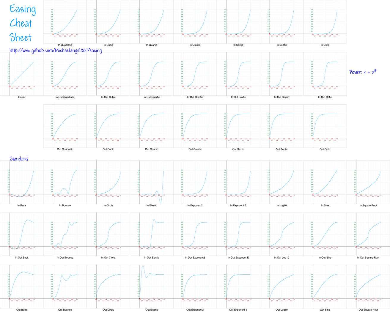
There is also a high resolution 4861x4000 Cheat Sheet

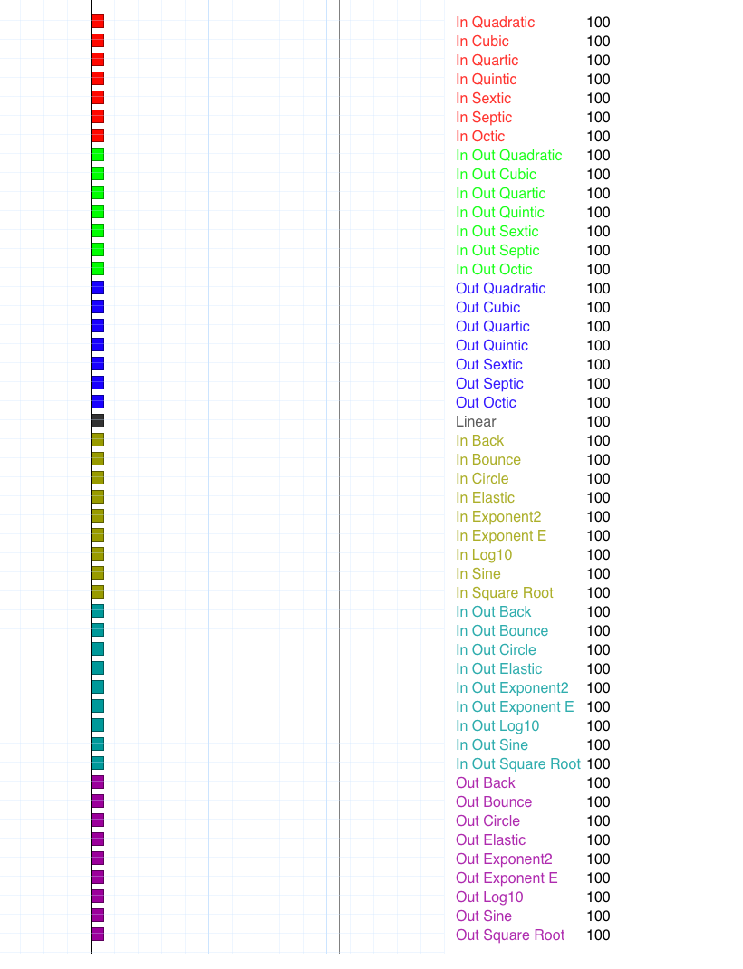
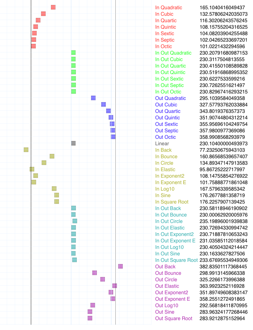
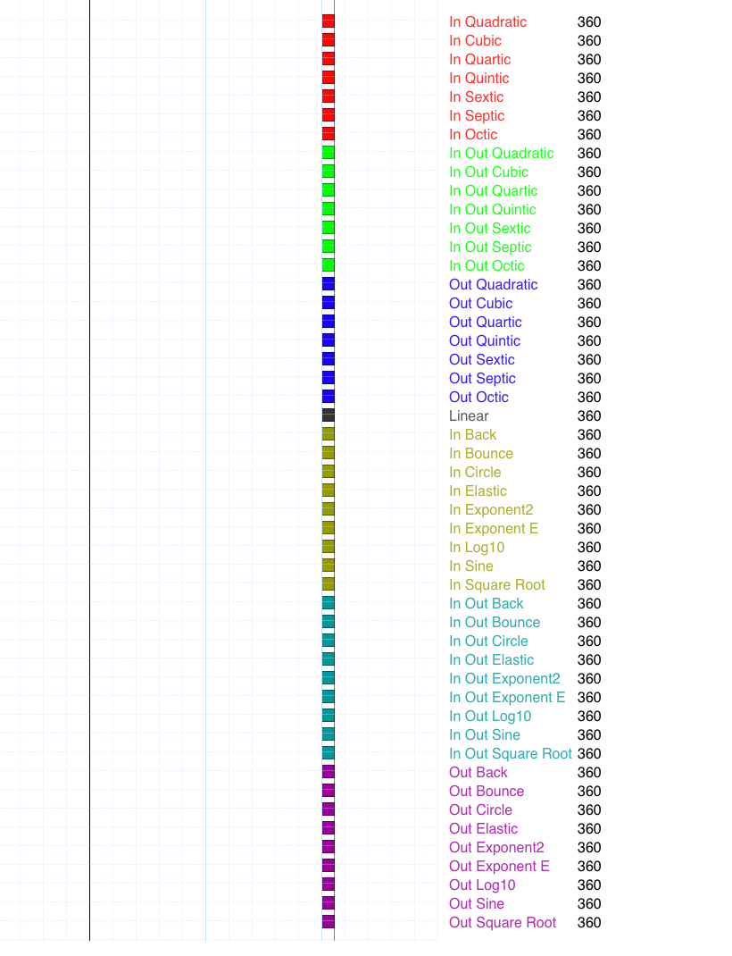
Comparision of easing functions

• Start of animation

• Middle of animation

• End of animation

TL:DR; “Shut up and show me the code!”

Jon Bentley has a talk called Three Beautiful Quicksorts sub-titled: “The most beautiful code I never wrote”

In contradistinction this is my “The most beautiful code I ever wrote.”

// Optimized Easing Functions by Michael "Code Poet" Pohoreski, aka Michaelangel007
// https://github.com/Michaelangel007/easing
// License: Free as in speech and beer; Attribution is always appreciated!
// Note: Please keep the URL so people can refer back to how these were derived.
var EasingFuncs = // Array of Functions
[
// Power -- grouped by In,Out,InOut
    function None           (p) { return 1;               }, // p^0 Placeholder for no active animation
    function Linear         (p) { return p;               }, // p^1 Note: In = Out = InOut
    function InQuadratic    (p) { return p*p;             }, // p^2 = Math.pow(p,2)
    function InCubic        (p) { return p*p*p;           }, // p^3 = Math.pow(p,3)
    function InQuartic      (p) { return p*p*p*p;         }, // p^4 = Math.pow(p,4)
    function InQuintic      (p) { return p*p*p*p*p;       }, // p^5 = Math.pow(p,5)
    function InSextic       (p) { return p*p*p*p*p*p;     }, // p^6 = Math.pow(p,6)
    function InSeptic       (p) { return p*p*p*p*p*p*p;   }, // p^7 = Math.pow(p,7)
    function InOctic        (p) { return p*p*p*p*p*p*p*p; }, // p^8 = Math.pow(p,8)

    function OutQuadratic   (p) { var m=p-1; return 1-m*m;             },
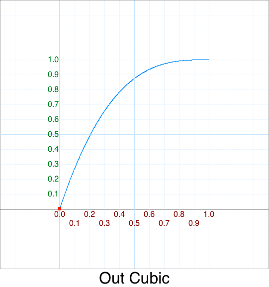
    function OutCubic       (p) { var m=p-1; return 1+m*m*m;           },
    function OutQuartic     (p) { var m=p-1; return 1-m*m*m*m;         },
    function OutQuintic     (p) { var m=p-1; return 1+m*m*m*m*m;       },
    function OutSextic      (p) { var m=p-1; return 1-m*m*m*m*m*m;     },
    function OutSeptic      (p) { var m=p-1; return 1+m*m*m*m*m*m*m;   },
    function OutOctic       (p) { var m=p-1; return 1-m*m*m*m*m*m*m*m; },

    function InOutQuadratic (p) { var m=p-1,t=p*2; if (t < 1) return p*t;             return 1-m*m            *  2; },
    function InOutCubic     (p) { var m=p-1,t=p*2; if (t < 1) return p*t*t;           return 1+m*m*m          *  4; },
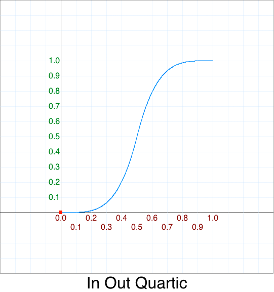
    function InOutQuartic   (p) { var m=p-1,t=p*2; if (t < 1) return p*t*t*t;         return 1-m*m*m*m        *  8; },
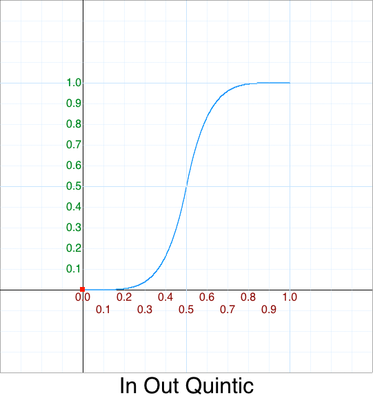
    function InOutQuintic   (p) { var m=p-1,t=p*2; if (t < 1) return p*t*t*t*t;       return 1+m*m*m*m*m      * 16; },
    function InOutSextic    (p) { var m=p-1,t=p*2; if (t < 1) return p*t*t*t*t*t;     return 1-m*m*m*m*m*m    * 32; },
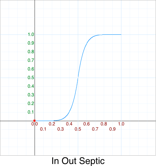
    function InOutSeptic    (p) { var m=p-1,t=p*2; if (t < 1) return p*t*t*t*t*t*t;   return 1+m*m*m*m*m*m*m  * 64; },
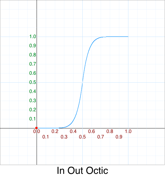
    function InOutOctic     (p) { var m=p-1,t=p*2; if (t < 1) return p*t*t*t*t*t*t*t; return 1-m*m*m*m*m*m*m*m*128; },

// Standard -- grouped by Type
    function InBack         (p) { var              k = 1.70158        ;              return p*p*(p*(k+1) - k);                                        },
    function InOutBack      (p) { var m=p-1,t=p*2, k = 1.70158 * 1.525; if (t < 1) return p*t*(t*(k+1) - k); else return 1 + 2*m*m*(2*m*(k+1) + k); }, // NOTE: Can go negative! i.e. p = 0.008
    function OutBack        (p) { var m=p-1,       k = 1.70158        ;                                             return 1 +   m*m*(  m*(k+1) + k); },

    function InBounce       (p) { return 1 - EasingFuncs[ Easing.OUT_BOUNCE ]( 1-p ); },
    function InOutBounce    (p) {
                                    var t = p*2;
                                    if (t < 1) return 0.5 - 0.5*EasingFuncs[ Easing.OUT_BOUNCE ]( 1 - t );
                                    return            0.5 + 0.5*EasingFuncs[ Easing.OUT_BOUNCE ]( t - 1 );
                                },
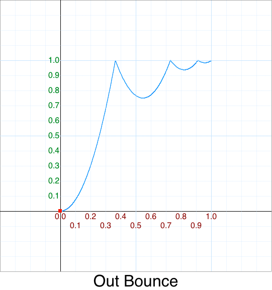
    function OutBounce      (p) {
                                    var r  = 1  / 2.75; // reciprocal
                                    var k1 =         r; // 36.36%
                                    var k2 = 2     * r; // 72.72%
                                    var k3 = 1.5   * r; // 54.54%
                                    var k4 = 2.5   * r; // 90.90%
                                    var k5 = 2.25  * r; // 81.81%
                                    var k6 = 2.625 * r; // 95.45%
                                    var k0 = 7.5625, t;

                                    /**/ if (p < k1) {             return k0 * p*p;            }
                                    else if (p < k2) { t = p - k3; return k0 * t*t + 0.75;     } // 48/64
                                    else if (p < k4) { t = p - k5; return k0 * t*t + 0.9375;   } // 60/64
                                    else             { t = p - k6; return k0 * t*t + 0.984375; } // 63/64
                                },

    function InCircle       (p) {                             return  1-Math.sqrt( 1 - p*p );                                                      },
    function InOutCircle    (p) { var m=p-1,t=p*2; if (t < 1) return (1-Math.sqrt( 1 - t*t ))*0.5; else return (Math.sqrt( 1 - 4*m*m ) + 1) * 0.5; },
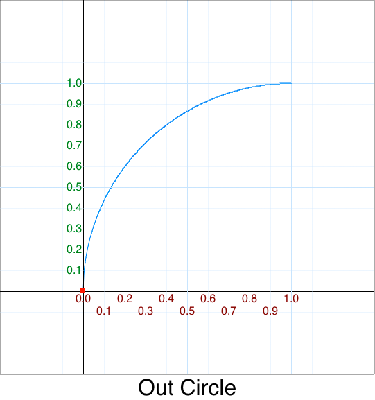
    function OutCircle      (p) { var m=p-1      ;                                                      return  Math.sqrt( 1 -   m*m );            },

    function InElastic      (p) { var m = p-1; return  - Math.pow( 2,10*m  ) * Math.sin( ( m*40 - 3) * Math.PI/6  ); },
    function InOutElastic   (p) {
                                    var s = 2*p-1;                 // remap: [0,0.5] -> [-1,0]
                                    var k = (80*s-9) * Math.PI/18; // and    [0.5,1] -> [0,+1]

                                    if (s < 0) return   -0.5*Math.pow(2, 10*s) * Math.sin( k );
                                    else       return 1 +0.5*Math.pow(2,-10*s) * Math.sin( k );
                                },
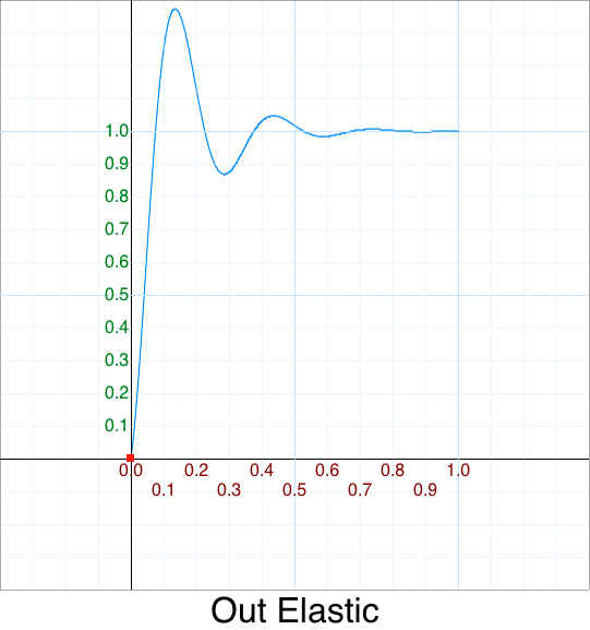
    function OutElastic     (p) {              return 1+(Math.pow( 2,10*-p ) * Math.sin( (-p*40 - 3) * Math.PI/6 )); },

    // NOTE: 'Exponent2' needs clamping for 0 and 1 respectively
    function InExponent2    (p) {   if (p <= 0) return 0; return   Math.pow( 2,  10*(p-1) ); },
    function InOutExponent2 (p) {
                                    if (p <= 0) return 0;
                                    if (p >= 1) return 1;
                                    if (p <0.5) return             Math.pow( 2,  10*(2*p-1)-1);
                                    else        return           1-Math.pow( 2, -10*(2*p-1)-1);
                                },
    function OutExponent2   (p)  {   if (p >= 1) return 1; return 1-Math.pow( 2, -10* p    ); },


    function InSine         (p) { return      1 - Math.cos( p * Math.PI*0.5 );  },
    function InOutSine      (p) { return 0.5*(1 - Math.cos( p * Math.PI     )); },
    function OutSine        (p) { return          Math.sin( p * Math.PI*0.5 );  },

// Non-Standard
    function InExponentE    (p) {   if (p <= 0) return 0; return   Math.pow( Math.E, -10*(1-p) ); }, // Scale 0..1 -> p^-10 .. p^0
    function InOutExponentE (p) {
                                    var t = p*2;
                                    if (t < 1) return 0.5 - 0.5*EasingFuncs[ Easing.OUT_EXPONENTE ]( 1 - t );
                                    return            0.5 + 0.5*EasingFuncs[ Easing.OUT_EXPONENTE ]( t - 1 );
                                },
    function OutExponentE   (p) { return 1 - EasingFuncs[ Easing.IN_EXPONENTE ]( 1-p ); },


    function InLog10        (p) { return 1 - EasingFuncs[ Easing.OUT_LOG10 ]( 1-p ); },
    function InOutLog10     (p) {
                                    var t = p*2;
                                    if (t < 1) return 0.5 - 0.5*EasingFuncs[ Easing.OUT_LOG10      ]( 1 - t );
                                    return            0.5 + 0.5*EasingFuncs[ Easing.OUT_LOG10      ]( t - 1 );
                                },
    function OutLog10       (p) { return Math.log10( (p*9)+1 ); }, // Scale 0..1 -> Log10( 1 ) .. Log10( 10 )

    function InSquareRoot   (p) { return 1 - EasingFuncs[ Easing.OUT_SQRT       ]( 1-p ); },
    function InOutSquareRoot(p) {
                                    var t = p*2;
                                    if (t < 1) return 0.5 - 0.5*EasingFuncs[ Easing.OUT_SQRT       ]( 1 - t );
                                    return            0.5 + 0.5*EasingFuncs[ Easing.OUT_SQRT       ]( t - 1 );
                                },
    function OutSquareRoot  (p) { return Math.sqrt( p ) },

    function Smoothstep(t,x0,x1){
        if( x0 === undefined ) x0 = 0;
        if( x1 === undefined ) x1 = 1;

        var p = (t - x0) / (x1 - x0);
        if( p < 0 ) p = 0;
        if( p > 1 ) p = 1;

        return p*p*(3-2*p);
    },
];

But we’re getting ahead of ourselves …

Easing … what is it and why is it important?

In UI (User Interface) design, UX (User Experience), or CG (Computer Graphics) rendering, often times we want to animate some “thing” over time. Basically “cheap physics” where cheap means inexpensive to calculate without resorting to a full physics simulation. For example:

• fade out an object (e.g. transistion alpha from 1.0 to 0.0),
• interpolate its location so it “slides offscreen” (e.g. change x (or y) over time), or
• the “reverse” animation of one of the above

Before we can do that we first need to know four things ..

• The start value
• The end value
• The duration of the animation
• The current elapsed time

… then we can calculate the current value. Once we have all the variables we can use this equation:

    current = start + (end-start)*(elapsed/duration);

The units of the initial start and final end values can be anything we wish as long as they all have the same consistent units. We could be animating something in px (pixels), over m/s (meters/second), etc. It doesn’t matter.

Likewise the duration and elapsed time could be in seconds, or milliseconds, etc., as long as we are again consistent and use the same units. Our calculations would be incorrect if we mixed the units – say duration was in seconds and elapsed in milliseconds. Hey, even rocket scientists sometimes have trouble with this concept in practice – don’t pull a NASA. :-)

For example, a designer wants us to animate a dialog panel from 30 pixels to 40 pixels over 10 seconds. We draw the screen at 60 times a second. What would be the current value (i.e. position) after 2 seconds?

Yes, this is a trivial example, but bear with me.

Our knowns:

start      = 30 px
end        = 40 px
elapsed    =  2 seconds
duration   = 10 seconds
frame rate = 60 Hz

Note: The frame rate was extraneous information. It never hurts to categorize ALL the information. We can always discard, or ignore, information that isn’t pertinent to the problem.

Anyways, solving for the unknown current position:

    position = start + (end-start)*(elapsed/duration);
    position = 30 + (2/10)*(40-30)
    position = 30 + (0.2*10)
    position = 30 + 2
    position = 32 px

If you don’t have an intuitive feel for what easing is then maybe this alternative analogy might help. Mathematically, easing is the same concept as calculating distance from Physics:

For example, when we have constant, linear motion we use the formula:

    Velocity = Distance/Time

And, solving for distance:

    Distance = Velocity*Time

Digressing slightly, in Physics Time, really is the Elapsed time, starting from zero. We’ll avoid sloppy ambigious terms like Time to minimize confusion.

Getting back on-topic. Note, that this is relative distance.

If we have an absolute start and end position the formula becomes:

    Position = Start + (End-Start)*(Elapsed/Duration)

Where did this formula come from?

We can replace Velocity with (Distance/Time) and re-solving for this new equation:

    Distance = Velocity*Time

    Position = Start + Velocity*Elapsed
    Position = Start + (Difference/Duration)*Elapsed
    Position = Start + (End-Start)*Elapsed

Notice how if start is zero the formula becomes the common:

    Position = 0 + (End-0)*(Elapsed/Duration)
    Position = End*(Elapsed/Duration)
    Distance = (End/Duration)*Elapsed
    Distance = Velocity*Elapsed
    Distance = Velocity*Time

Now as programmers we love to invent our own terminology.

However, instead of a “hard-coded” formula we:

1. we call animation the name “easing”, and
2. parameterize it.

What the heck is Parameterization ?

Parameterization is just a fancy word for abstraction or generalizing. Instead of using a hard-coded fixed function we instead use a generic or custom function. We’ll discuss this more later.

Remember, our easing formula looks like:

    position = start + (end - start)*(elapsed/duration);

As a function, it might look like:

    Easing: function( ... )
    {
        var position = ...;
        return position;
    }

With parameterization, it might look like:

    Easing: function( type, ... )
    {
        var position;

        switch( type )
        {
            case FOO: position = ...; break;
            case BAR: position = ...; break;
            case QUX: position = ...; break;
            default: console.error( "ERROR: Unknown easing type" );
        }

        return position;
    }

Since arrays of Javascript are associate arrays we can remove that switch statement:

    Easings = {
        foo: function( ... ) { return ...; },
        bar: function( ... ) { return ...; },
        qux: function( ... ) { return ...; },
    };

    Easing: function( type, ... )
    {
        return Easings[ type ]( ... );
    }

But before we can calculate the final position we need the relevent information:

    position = Easing( type, progress, start, end )

Where progress = elapsed/duration

We’ll get to easing types shortly but first we need to talk about time.

Parameter t or p

That elapsed / duration term is kind of clunky.

For convenience we normalize time to be a normalized percentage of the elapsed time. Now that is a bit of a mouthful, so let’s break it down into simpler terms:

• Percentage means between 0% and 100%,
• Normalized in this context means between 0.0 and 1.0. Mathematically the range is [0,1], that is, between 0.0 (inclusive) and 1.0 (inclusive). See my StackOverflow answer about What does the square bracket and parenthesis mean?

Since normalized percentage is so common and unweildy most people just use the shorted phrase: normalized

If you are familiar with OpenGL or DirectX graphic API’s, when a vertex is transformed through the pipeline you will run across something called “Normalized Device Coordinates” which embody the same idea.

If we wanted to place an object at the middle of the screen we could place its center point at:

• <screen width/2, screen height/2, 0.0> (in pixels),

OR, in normalized coordinates:

• <0.5, 0.5> – basically half the width, and half the height.

Getting back to our normalized time value p …

    p = elapsed / duration.

What does this mean? You could think of p being a mnemonic for progress. Visually when p is:

p	Animation …
0.0	… has not yet started – the object is still at its initial value
0.5	… is half way done
1.0	… is complete – the object has reached its final value

Note: Often you’ll see the paramater name t in formulas. I’ll avoid it since it can be confused with time which may or may not be normalized. UGH.

Instead, I’ll use the variable p as a visual mnemonic that we are representing a normalized percentage elapsed time, that is, elapsed/duration.

Simultaneous Animations

There is no reason why we couldn’t even have multiple simultaneous animations on the same object all going on at once! Typically objects have more than one dimension, such as eight dimensions (8D).

Eight dimensions!?

Whoa! Where did all those come from? When did this turn into String Theory? :-)

Relax, we’re not talking about the esoteric nature of reality, only simulating some of the useful bits, pardon the pun.

For example we could have:

• an object starts faded out (alpha = 0.0),
• is offscreen (start x = -width of object),
• starts small (start width & height = 1 px)
• slides in to the center of the screen (final x = screen width/2), and
• becomes opaque (alpha = 1.0)
• grows to half size (end width = screen width/2 px, end height = screen height/2 px)

These animation or easing axis are all independent. We could represent these axis in Javascript as:

var Axis =
{
    X   : 0, // left position    (in pixels)
    Y   : 1, // top  position    (in pixels)
    W   : 2, // width  dimension (in pixels)
    H   : 3, // height dimension (in pixels)
    R   : 4, // normalized red   color
    G   : 5, // normalized green color
    B   : 6, // normalized blue  color
    A   : 7, // normalized alpha color
    NUM : 8,
};

Why Javascript?

Javascript (JS) is a crappy (*) language designed in 10 days. If it is so bad then why use it?

Two reasons:

• Every modern computer has a web browser which means there is nothing to install, and
• More importantly, to show that it is possible to write good (**) code in any language, even as one as bad as Javascript.

(*) What precisely makes Javascript so garbage you ask?

• It is BASIC all over again – accidently misspell a variable and JS uses the undefined value without any warnings …
• … unless you use the hack "use strict"; at the top of every Javascript program
• No ability to include other code – unless you use require hack which only works in server and not in a browser
• ASI, aka Automatic Semicolon Insertion. You can’t put a return on a line by itself due to the idiotic grammar/parsing. Douglas Crockford said it best @3:41 “Why am I betting my career on this piece of crap?”
• No native unsigned 64-bit int. var n = (1 << 63); console.log( n ); // -2147483648 // facepalm
• Every number is a 64-bit floating-point, unless you use Float32Array
• The comparision operator == is horribly broken i.e. if( 0 == "0" ) console.log( "equal" ); // equal!?
• Its type system is foobar. See Gary Bernhardt’s WAT talk for how brain-dead JS is. No, not that language.
• No automatic multiline string concatenation. This means you need to do stupid shit like this at run-time:

 var text = 'First line\n'
          + 'Second line\n'
          + 'Third line\n'
          ;

instead of C’s automatic multiline string concatenation:

   char *text =
"First line\n"
"Second line\n"
"Third line\n"
        ;

or Python’s way:

    s = """ First Line
            Second line
            Third line """

Of course you have to deal with Python’s idiotic indentation shenanigans but that is a discussion for another day.

(**) Good code is one that has:

• succinct and descriptive variable names,
• lots of whitespace (both horizontally and vertically),
• uses multi-column alignment
• documents WHY not HOW

An example of how to write GOOD code: widget.js

Example of how NOT to write code: procmail.c

OK, enough ranting. Let’s get back to our axis of evil, er, 8D axis …

The Color Axis

The astute reader will notice I snuck color in there!

i.e. What if we wanted to fade an object from Black to Yellow and back to Black again, say for a glowing highlight? By separating the hue into separate axis such as red, green, and blue, our animation engine could support this very easily.

Why seperate the axis?

We may be given two colors in a hex string format, #RRGGBB, and want to interpolate between them. Before we can do this we would need to

• Break this down into the 3 components, or Red, Green, Blue axis, respectively.
• Then we need to scale the triad (between 0 and 255), and
• Combine them to form a valid #RRGGBB hex string.
• Lastly, we need to apply the color to the HTML element.

For example this function will do exactly the middle part.

// Convert numeric r,g,b values to an HTML color hex string `#RRGGBB`
function RGBtoHex = function( r, g, b )
{
    return '#'
        + ('0' + ((255 * r) | 0).toString( 16 )).slice( -2 )
        + ('0' + ((255 * g) | 0).toString( 16 )).slice( -2 )
        + ('0' + ((255 * b) | 0).toString( 16 )).slice( -2 )
};

Sometimes you’ll see the terminology of a controller.

i.e. If we wanted to animate across the rainbow from Red, Orange, Yellow, Green, Cyan, Azure, Blue, Violet, Magenta it might be more convenient to use a hue controller.

At the high level it would be:

    /** Animate between two colors
     *  @param {Number} startAngle - starting color in degrees
     *  @param {Number} endAngle   - end      color in degrees
     *  @param {Number} duration   - duration in seconds
     */
    function HueControllerAnimate( startAngle, endAngle, duration )
    {
        // Animate an angle from startAngle to endAngle over a duration
        // On each update
        //    convert hue to r,g,b
        //    apply it to the object
    }

This would in turn drive the animation values red, green, blue over time.

The reason I bring up color is that if you start interpolating color you may need to look into PMA (Premultiplied alpha) – where you need to multiply alpha into the red, green, and blue channels.

See Tom Forsyth’s Blog for these 2 articles:

• Premultiplied alpha, 18 March 2015 (created 15 July 2006)
• Premultiplied alpha part 2, 18 March 2015 (created 18 March 2015)

But I digress.

Linear Interpolation: Lerp

In computer graphics terminology this calculating “inbetween” values is called interpolation. In animation it is called tweening.

Given different times, we want these values:

p	Value
0.0	start
0.5	0.5*(end-start)
1.0	end

What we have just discussed is the simplist type of interpolation: a linear interpolation.

The graph looks like this:

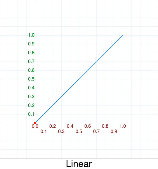
Since this type of interpolation is so common it has its own abbreviation: Lerp

• “Lerp” - linear interpolation.

Lerp is typically shown in one of two common forms:

    function lerp( t, a, b )
    {
        return a + (t-1)(b-a);
    }

or

    function lerp( t, a, b )
    {
        return (1-t)*a + t*b;
    }

This is one of those times where t is commonly used.

Let’s replace those abbreviations with descriptive names for now since we want to understand what they mean.

    function lerp( p, start, end )
    {
        return start + (p-1)(end-start);
    }

    function lerp( p, start, end )
    {
        return (1-p)*start + p*end;
    }

Note: Some programmers factor out (end-start) and call it c for change or d for delta but with the latter d could also mean duration so be aware of different conventions used by people.

Mathematically, the two lerp equations are equivalent but since computers are finite they have precision errors which can and do creep in. You should be familiar with both forms as you’ll see them in common usage.

The first one in practice may not be as accurate as the latter due to floating-point error accumulation. Why would it be used then? The first form is popular due to modern hardware often having a native FMA Fused Multiply-Add hardware instruction. Thus sometimes you’ll see the second form to maximize precision and minimize error, at the cost of slightly slower performance.

This is a common trade-off in computing – you can have speed or accuracy, pick one. :-/

Non-linear interpolation: slerp

If one interpolates between two quaternions they will come across the term slerp.

This is just an abbreviation for spherical interpolation.

Quaternions won’t be discussed here, but it is also nice to be aware of the broader terminology in related fields.

Non-linear interpolation: smoothstep

In computer graphics there is a common (cubic) interpolation function called Smoothstep():

smoothstep function( t, x0, x1 )
{
    var p = (t - x0) / (x1 - x0);

    if( p < 0 ) p = 0;
    if( p > 1 ) p = 1;

    return p*p*(3-2*p);
}

The graph looks like this:

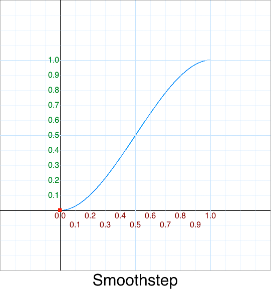
See my interactive WebGL smoothstep demo.

De Facto Easing Functions

Back in 2001 Robert Penner provided the original, “canonical” de facto easing functions written in ActionScript. They became extremely popular.

First, let’s tabulate the arguments they use:

Legend:

Symbol	Meaning	Notes
x	not used	Useless extra argument that just clutters up the code
t	elapsed time	Starting from zero
b	begin val
c	change val	end-begin
d	duration	BUG: generates NaN if zero!

And without further ado:

// http://www.robertpenner.com/easing
// by Robert Penner Copyright 2001
// License: BSD -- http://robertpenner.com/easing_terms_of_use.html
// http://robertpenner.com/easing/penner_easing_as1.txt

Math.linearTween = function (t, b, c, d) { // Page 202
    return c*t/d + b;
};

Math.easeInQuad = function (t, b, c, d) { // Page 210
    return c*(t/=d)*t + b;
};

Math.easeOutQuad = function (t, b, c, d) { // Page 211
    return -c * (t/=d)*(t-2) + b;
};

Math.easeInOutQuad = function (t, b, c, d) { // Page 211
    if ((t/=d/2) < 1) return c/2*t*t + b;
    return -c/2 * ((--t)*(t-2) - 1) + b;
};

Math.easeInCubic = function (t, b, c, d) { // Page 212
    return c * Math.pow (t/d, 3) + b;
};

Math.easeOutCubic = function (t, b, c, d) { // Page 212
    return c * (Math.pow (t/d-1, 3) + 1) + b;
};

Math.easeInOutCubic = function (t, b, c, d) { // Page 212
    if ((t/=d/2) < 1)
        return c/2 * Math.pow (t, 3) + b;
    return c/2 * (Math.pow (t-2, 3) + 2) + b;
};

Math.easeInQuart = function (t, b, c, d) { // Page 213
    return c * Math.pow (t/d, 4) + b;
};

Math.easeOutQuart = function (t, b, c, d) { // Page 213
    return -c * (Math.pow (t/d-1, 4) - 1) + b;
};

Math.easeInOutQuart = function (t, b, c, d) { // Page 213
    if ((t/=d/2) < 1)
        return c/2 * Math.pow (t, 4) + b;
    return -c/2 * (Math.pow (t-2, 4) - 2) + b;
};

Math.easeInQuint = function (t, b, c, d) { // Page 214
    return c * Math.pow (t/d, 5) + b;
};

Math.easeOutQuint = function (t, b, c, d) { // Page 214
    return c * (Math.pow (t/d-1, 5) + 1) + b;
};

Math.easeInOutQuint = function (t, b, c, d) { // Page 214
    if ((t/=d/2) < 1)
        return c/2 * Math.pow (t, 5) + b;
    return c/2 * (Math.pow (t-2, 5) + 2) + b;
};

Math.easeInSine = function (t, b, c, d) { // Page 215
    return c * (1 - Math.cos(t/d * (Math.PI/2))) + b;
};

Math.easeOutSine = function (t, b, c, d) { // Page 215
    return c * Math.sin(t/d * (Math.PI/2)) + b;
};

Math.easeInOutSine = function (t, b, c, d) { // Page 215
    return c/2 * (1 - Math.cos(Math.PI*t/d)) + b;
};

Math.easeInExpo = function (t, b, c, d) { // Page 216
    return c * Math.pow(2, 10 * (t/d - 1)) + b;
};

Math.easeOutExpo = function (t, b, c, d) { // Page 216
    return c * (-Math.pow(2, -10 * t/d) + 1) + b;
};

Math.easeInOutExpo = function (t, b, c, d) { // Page 216
    if ((t/=d/2) < 1)
        return c/2 * Math.pow(2, 10 * (t - 1)) + b;
    return c/2 * (-Math.pow(2, -10 * --t) + 2) + b;
};

Math.easeInCirc = function (t, b, c, d) { // Page 218
    return c * (1 - Math.sqrt(1 - (t/=d)*t)) + b;
};

Math.easeOutCirc = function (t, b, c, d) { // Page 218
    return c * Math.sqrt(1 - (t=t/d-1)*t) + b;
};

Math.easeInOutCirc = function (t, b, c, d) { // Page 218
    if ((t/=d/2) < 1)
        return c/2 * (1 - Math.sqrt(1 - t*t)) + b;
    return c/2 * (Math.sqrt(1 - (t-=2)*t) + 1) + b;
};

Math.easeInBounce = function (t, b, c, d) {
    return c - Math.easeOutBounce (d-t, 0, c, d) + b;
};

Math.easeOutBounce = function (t, b, c, d) {
    if ((t/=d) < (1/2.75)) {
        return c*(7.5625*t*t) + b;
    } else if (t < (2/2.75)) {
        return c*(7.5625*(t-=(1.5/2.75))*t + .75) + b;
    } else if (t < (2.5/2.75)) {
        return c*(7.5625*(t-=(2.25/2.75))*t + .9375) + b;
    } else {
        return c*(7.5625*(t-=(2.625/2.75))*t + .984375) + b;
    }
};

Math.easeInOutBounce = function (t, b, c, d) {
    if (t < d/2) return Math.easeInBounce (t*2, 0, c, d) * .5 + b;
    return Math.easeOutBounce (t*2-d, 0, c, d) * .5 + c*.5 + b;
};

Math.easeInBack = function (t, b, c, d, s) {
    if (s == undefined) s = 1.70158;
    return c*(t/=d)*t*((s+1)*t - s) + b;
};

Math.easeOutBack = function (t, b, c, d, s) {
    if (s == undefined) s = 1.70158;
    return c*((t=t/d-1)*t*((s+1)*t + s) + 1) + b;
};

Math.easeInOutBack = function (t, b, c, d, s) {
    if (s == undefined) s = 1.70158;
    if ((t/=d/2) < 1) return c/2*(t*t*(((s*=(1.525))+1)*t - s)) + b;
    return c/2*((t-=2)*t*(((s*=(1.525))+1)*t + s) + 2) + b;
};

Math.easeInElastic = function (t, b, c, d, a, p) {
    if (t==0) return b;  if ((t/=d)==1) return b+c;  if (!p) p=d*.3;
    if (a < Math.abs(c)) { a=c; var s=p/4; }
    else var s = p/(2*Math.PI) * Math.asin (c/a);
    return -(a*Math.pow(2,10*(t-=1)) * Math.sin( (t*d-s)*(2*Math.PI)/p )) + b;
};

Math.easeOutElastic = function (t, b, c, d, a, p) {
    if (t==0) return b;  if ((t/=d)==1) return b+c;  if (!p) p=d*.3;
    if (a < Math.abs(c)) { a=c; var s=p/4; }
    else var s = p/(2*Math.PI) * Math.asin (c/a);
    return a*Math.pow(2,-10*t) * Math.sin( (t*d-s)*(2*Math.PI)/p ) + c + b;
};

Math.easeInOutElastic = function (t, b, c, d, a, p) {
    if (t==0) return b;  if ((t/=d/2)==2) return b+c;  if (!p) p=d*(.3*1.5);
    if (a < Math.abs(c)) { a=c; var s=p/4; }
    else var s = p/(2*Math.PI) * Math.asin (c/a);
    if (t < 1) return -.5*(a*Math.pow(2,10*(t-=1)) * Math.sin( (t*d-s)*(2*Math.PI)/p )) + b;
    return a*Math.pow(2,-10*(t-=1)) * Math.sin( (t*d-s)*(2*Math.PI)/p )*.5 + c + b;
};

Uhm, yeah. NOT.

Let’s learn how to clean up this fugly, overengineered code into the beautiful, exact equivalent mentioned at the beginning.

The astute reader will notice that jQuery initially adapted these “as-is” before coming to their senses and cleaning them up into the single parameter version.

• https://raw.githubusercontent.com/danro/jquery-easing/master/jquery.easing.js

Easing Cleanup

There are numerous problems with the defacto 5-parameter easing functions. This is crap code – that’s the “technical” term for over-engineered.

Problems can be placed into two general categories:

• Meta
• Implementation

The meta coding problems are:

• Functions aren’t alphabetized making searching/finding them non-intuitiave.
• While inter-easing functions are grouped together there is no seperator between intra-easing such as whitespace.
• Names are abbreviated making them not obvious, such as Expo – Exponent comes in multiple variations such as Exponent_2 and Exponent_e.
• Initially there seems to be a lot of easing functions, but they are incomplete – they are missing some of the more common mathematical ones.

The implementation problems are:

1. Buggy 1 - Generates NaN when d == 0
2. Buggy 2 - Doesn’t handle edge cases when t < 0 or t > d
3. Inefficient - t/d is always done to normalize the time; If there are multiple animations with the same duration then this causes extra processing. Also, you can often multiply by the reciprocal duration instead of doing a slow divide. When the animation is started we “pre-calculate” 1/duration.
4. Slow 1 - due to inefficient, redundant, or dead code
5. Slow 2 - b can be replaced with 0.0
6. Slow 3 - c can be replaced with 1.0
7. Wasteful - Some versions have an extra first argument x declared in all functions but is never used

We will address and fix all of these bugs.

Cleanup - Linear

First, let’s start with the linear easing.

Hmm, there isn’t one. Really?! Let’s add one for completeness.

Recall its graph looks like this:

And in the original style the easing function would look like this:

    easeLinear: function (x, t, b, c, d) {
        return c*(t/=d) + b;
    },

Now, when d is 0, this generates a bug #1 NaN. Let’s digress slightly and address bug #2, t < 0 and t > d before we fix this.

    easeLinear: function (x, t, b, c, d) {
        if (t <= 0) return b    ; // start
        if (t >= d) return b + c; // end
        return c*(t/=d) + b;

What happens when d is zero ? It returns the end for free!

    easeLinear: function (x, t, b, c, d) {
        if (t <= 0) return b    ;
        if (t >= d) return b + c; // t >= 0 return end
        return c*(t/=d) + b;

Let’s make this a little more robust:

    easeLinear: function (x, t, b, c, d) {
        if (t <= 0) return b    ; // If d=0, then t is always t >= d
        if (t >= d) return b + c; // due to t < 0 already being handled
        var p = t/d;
        return c*p + b;
    },

Hmmm, some of these equations are starting to look familiar !

“I’m here for an argument”

Without being pedantic with Argument vs Parameter we still have a lot of parameters in our easing functions. Is there any way we can get rid of them? Yes, with reparameterization.

Reparameterization is just a fancy word for re-mapping. Technically, it is this.

There will be a test. :)

Since that Wikipedia page is so badly written – and will probably just confuse you more than it helps – the only take-away you need is this:

• Reparameterization … is the process of deciding and defining the parameters necessary for a … specification.

A simple mnemonic to help remember is: re-parameter

Basically, we want to re-map the range into something convenient. But that raises the question – what would be convenient? Hmm, since we can pick any start and end values – maybe a range between 0.0 and 1.0 (inclusive) aka normalized values? :) Whoever calls us will be responsible for scaling the values back up to their full range.

b	c	Notes
min	max-min	Old range
0.0	1.0	New range

    easeLinear: function (x, t, b, c, d) {
        if (t <= 0) return b    ; // If d=0, then t is always t >= d
        if (t >= d) return b + c; // due to t < 0 already being handled
        var p = t/d;
        return c*p + b;
    },

Becomes

    easeLinear: function (x, t, d) {
        if (t <= 0) return 0; // If d=0, then t is always t >= d
        if (t >= d) return 1; // due to t < 0 already being handled
        var p = t/d;
        return p;
    },

Notice now:

• how the term b drops out from the arguments,
• how the term c drops out from the arguments,
• The entire formula becomes much simpler.

We’ll do this for all the original easing equations converting them into a single argument version using these steps:.

1. Since x is unused our function prototype becomes: function( t, b, c, d )
2. Since b is zero, our function prototype becomes: function( t, c, d )
3. Since c is one, our function prototype becomes: function( t, d )
4. Whoever calls our easing function will be responsible for the p = t/d calculation so we can remove the last two terms and replace them with one.

Our function prototype then is the simple:

function Linear( p ) {
    return p;
}

We’ll also drop the ease prefix since:

• These functions will be in a namespace anyways, and
• It provides a visual mnemonic to know which easing functions take 1 argument vs 5 arguments. If the function starts with ease it is the 5 parameter version. If the function doesn’t start with ease then we know it is the 1 parameter version.

“Warp Speed, Mr. Sulu”

Now this linear easing form by itself isn’t very interesting.

However, what if we adjusted the time ? That is, when the animation is:

• 0% done, no change,
• 10% done, we pretend it is only 1% done,
• 20% done, we pretend it is only 4% done,
• 30% done, we pretend it is only 9% done,
• 40% done, we pretend it is only 16% done,
• 50% done, we pretend it is only 25% done,
• 60% done, we pretend it is only 36% done,
• 70% done, we pretend it is only 49% done,
• 80% done, we pretend it is only 64% done,
• 90% done, we pretend it is only 81% done,
• 100% done, it really is 100% done.

Spot the pattern?

Using this legend:

• x = Percent ‘normal’ time
• y = Percent ‘warped’ time

Here is the data in table format:

x	y
0.0	0.00
0.1	0.01
0.2	0.04
0.3	0.09
0.4	0.16
0.5	0.25
0.7	0.49
0.8	0.64
0.9	0.81
1.0	1.00

If we graph this pretend game we end up with this:

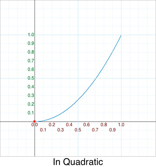
This is what is known as a quadratic mapping.

Mathematically the formula looks like this:

    y = x*x

Or in our parlance:

    function InQuadratic(p) { return p*p; }, // p^2 = Math.pow(p,2)

In one sense you could say that easing is a function that “warps time”. We can apply all sorts of “time warping” to produce many different interesting effects.

But before we investigate and optimize them we first need to go over the concepts of:

• In,
• Out, and
• In Out

“What’s up with this ‘In’, ‘Out’, ‘In-Out’ business, anyways?”

We introduced a new easing function which has the form of a Quadratic equation:

    function InQuadratic(p) { return p*p; }

And its graph:

We have p^2, but what about raising p to the standard (integer) powers such as 3, 4, 5, …, etc.? Here are the common names for polynomials of degree n:

Power	Formula	Name
1	p^1	Linear
2	p^2	Quadratic
3	p^3	Cubic
4	p^4	Quartic
5	p^5	Quintic
6	p^6	Sextic
7	p^7	Septic
8	p^8	Octic

Those graphs look like these:

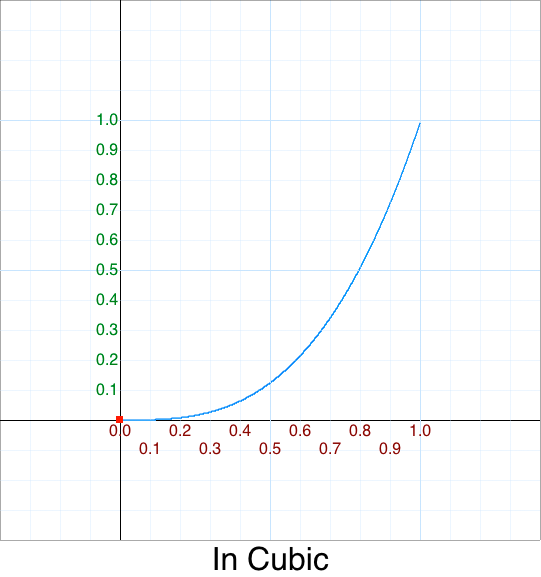
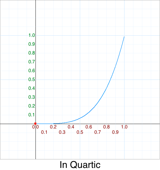
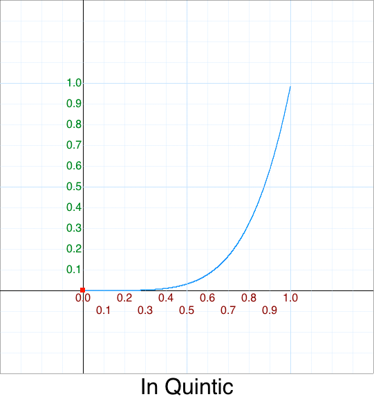
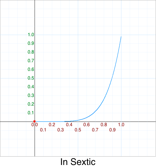
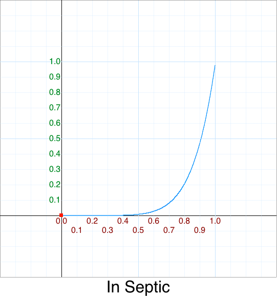
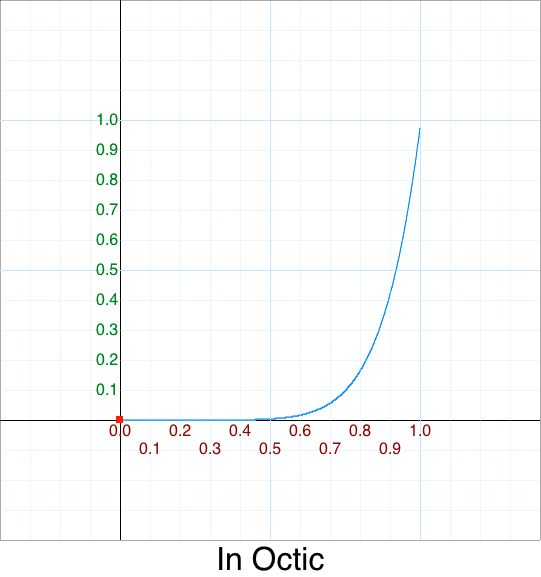
We’ll discuss other variations later.

Out

You may have noticed we snuck in the prefix In but didn’t have one for Linear.

• Linear
• InQuadratic
• InCubic
• InQuartic
• etc.

There are two reasons for that:

• Linear doesn’t have them – once you finish this section you’ll understand why.
• If you assumed this implies there are more variations you would be correct! There are many variations of mirrors, rotations, etc.

Now the linear line is a constant motion. Anything below the line we call an In

And anything above the linear line we call an Out

For now we’re primarily interested in mirroring along the principal axis or what I will call flips – of which there are 4 permutations:

“No backflip for you!”

1. We have already been discussing the case of no flips.

Flip Y

2. What happens when we flip the output along the y-axis:

    function FlipY_Quadratic(p) { return 1 - InQuadratic( p ); }

That has a graph that looks like this:

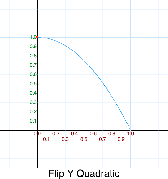
Flip X

1. We could also flip the input along the x-axis:

     function FlipX_Quadratic(p) { return InQuadratic( 1-p ); }

That has a graph that looks like this:

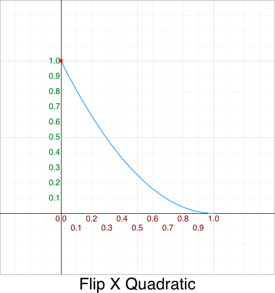
Flip X, Flip Y

1. The most interesting is is when we flip along both the x-axis and y-axis:

     function FlipY_FlipX_Quadratic(p) { return 1 - InQuadratic( 1-p ); }

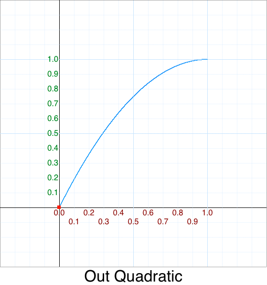
This pattern of both x and y being flipped is so common that it has its own name: Out

     function OutQuadratic(p) { return 1 - InQuadratic( 1-p ); }

Now you may be thinking “That doesn’t even look like the one I saw at the very top!?”

i.e. To refresh your memory:

    function OutQuadratic (p) { var m=p-1; return 1-m*m; }

Let’s “semantically uncompress” this adding line breaks and whitespace so it is more readable:

    function OutQuadratic (p)
    {
        var m = p-1;

        return 1 - m*m;
    }

Mathematically, the two are exact; the original function has just been optimized so that the general pattern of the power series can be easier to spot

I’ll discuss in the Clean Up - Out Quadratic section, etc.

For recap we derived 4 quadratic easing functions:

    function      QuadraticIn      (p) { return        p *   p ; } // Red
    function FlipXQuadraticIn      (p) { return     (1-p)*(1-p); } // Green
    function FlipYQuadraticIn      (p) { return 1 -    p *   p ; } // Blue
    function FlipYFlipXQuadraticIn (p) { return 1 - (1-p)*(1-p); } // Orange "OutQuadratic"

If you want to play around with these, there is an excellent online (browser) graphing calculator: Desmos

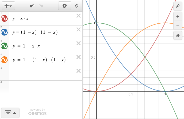
I’ve added color names to the above flip functions so you can see what corresponds to what since I’m not aware if you can name functions in Desmos.

This reminds me of the Cubic Hermite spline – specifically, the hermite basis functions.

I mentioned that there is an Out variation for Linear. By now it should be obvious that the FlipYFlipX for Linear doesn’t change its graph. Specifically,

• InLinear = OutLinear

Just in case you were wondering now you know.

In-Out

In addition to flips there is also another variation called InOut where we “stitch” together both the In and Out into one continuous function.

This means we need to move 2 points:

• The end-point of In from <1,1> to <0.5,0.5>
• The start-point of Out from <0,0> to <0.5,0.5>

This requires 5 pre-requisites:

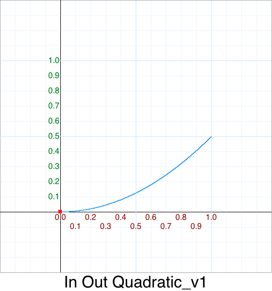
1. Scale the In height (y) by 1/2.

function InOutQuadratic_v1( p ) {
    return 0.5 * InQuadratic( p );
}

or simply when inlined:

function InOutQuadratic_v1( p ) {
    return 0.5 * p*p;
}

That graph looks like this:

1. Scale the In width (x) by 1/2.

How? Reparameterization to the rescue! We can remap our original input p range and split it into two ranges. I’ll call the new input t:

old p input	new t input
[0.0 .. 0.5)	[0.0 .. 1.0]
[0.5 .. 1.0]	don’t care

And with a little bit of algebra it should be obvious of the scale factor:

    Input  : p = [0.0 .. 0.5)
    Output : t = [0.0 .. 1.0]
    Formula: t = 2*p

function InOutQuadratic_v2( p ) {
    var t = 2*p;
    return 0.5 * InQuadratic( t );
}

or when inlined:

function InOutQuadratic_v2( p ) {
    return 0.5 * (2*p)*(2*p);
}

Which simplifies down to:

function InOutQuadratic_v2( p ) {
    return 2 * (p*p);
}

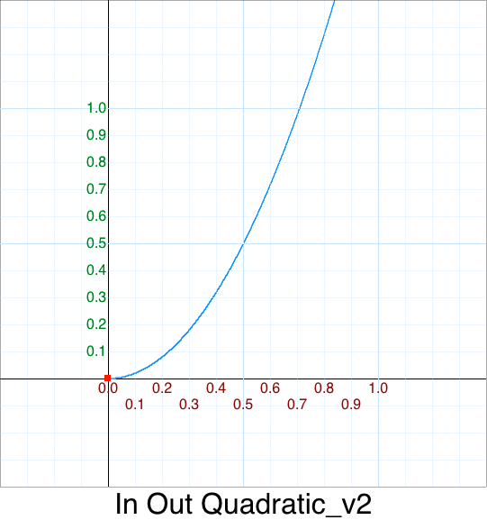
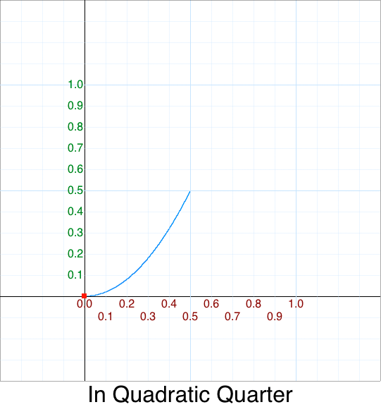
What we have done is move the end-point of In at <1,1> to <0.5, 0.5>. Since we are only keeping the bottom quarter we don’t care about the right side of the graph as we’ll replace that with the Out form.

3. Similiarly for In we scale the Out height (y) by 1/2

 function InOutQuadratic_v3( p ) {
     return 0.5 * OutQuadratic( p );
 }

or when inlined:

 function InOutQuadratic_v3( p ) {
     return 0.5 * (1 - ((1-p)*(1-p)));
 }

The graph looks like this:

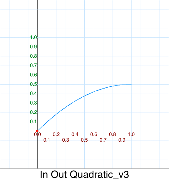
4. Again, similiarly for In we scale the Out width (x) by 1/2

Using reparameterization again we remap our original input p range and split it into two ranges. Again, I’ll call the new input t:

p range	new t range
[0.0 .. 0.5)	don’t care
[0.5 .. 1.0]	[0.0 .. 1.0]

Solving for t:

    Input  : p = [0.5 .. 1.0]
    Output : t = [0.0 .. 1.0]
    Formula: t = 2*p-1

Leaving:

function InOutQuadratic_v4( p ) {
    var t = 2*p - 1;
    return 0.5 * OutQuadratic( 2*p - 1 );
}

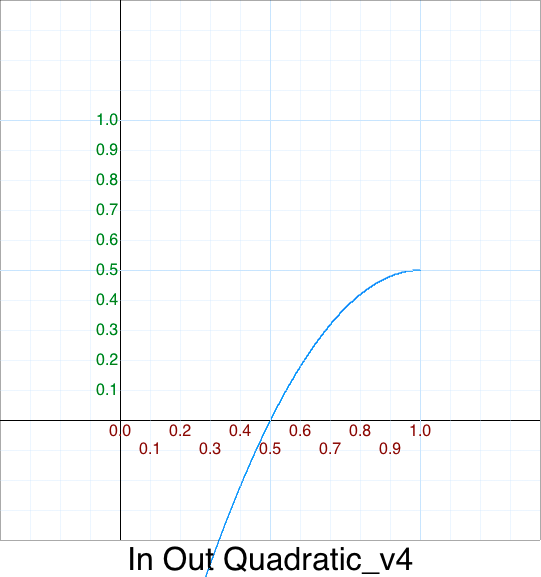
We’ll simplify this later in the Cleanup - In Out Quadratic section.

Again, we don’t care about the left side since that is being replaced with In

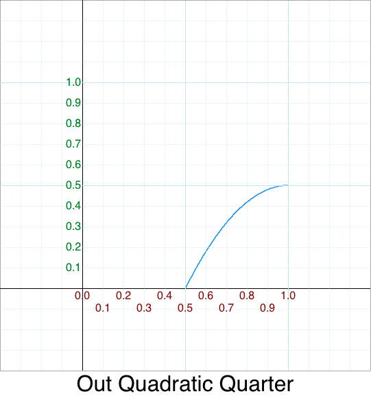
5. We need to move the <0,0> of Out to <0.5,0.5>

That is done by simply shifting the graph “up”, via y + 0.5

function InOutQuadratic_v5( p ) {
    var t = 2*p - 1;
    return 0.5 + 0.5*OutQuadratic( 2*p - 1 );

    //           \_________________________/
    //     0.5 +           y
}

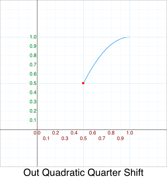
And now we can piece together our InOut function.

First the In:

function InOutQuadratic_v2( p ) {
    var t = 2*p;
    return 0.5 * InQuadratic( t );
}

Plus the Out:

function InOutQuadratic_v5( p ) {
    var t = 2*p - 1;
    return 0.5 + 0.5*OutQuadratic( 2*p - 1 );
}

In Mathematics this is called a piecewise function.; it is written with the curly brace notation:

y =       0.5*InQudratic  ( 2*x     )   { 0  < x <= 1/2 }
y = 0.5 + 0.5*OutQuadratic( 2*x - 1 )   {1/2 < x <= 1   }

or alternatively:

    {        0.5*InQudratic  ( 2*x     ), if x <  1/2
y = {
    {  0.5 + 0.5*OutQuadratic( 2*x - 1 ), if x >= 1/2

We can factor out the common term 2*x as t (for two times) for readability:

function InOutQuadratic_v6( p )
{
    var t = 2*p;

    if( p < 0.5 ) return       0.5*InQuadratic ( t     );
    else          return 0.5 + 0.5*OutQuadratic( t - 1 );
}

Since the end point of the In is the start point of Out, that is , (p <= 0.5) is equivalent to (p < 0.5) We can remove some visual clutter by removing that 0.5 and use 1 directly

function InOutQuadratic_v6( p )
{
    var t = 2*p;

    if( t < 1 ) return       0.5*InQuadratic ( t     );
    else        return 0.5 + 0.5*OutQuadratic( t - 1 );
}

And now for the moment of truth:

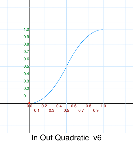
TA-DA !

This matches our optimized version: :)

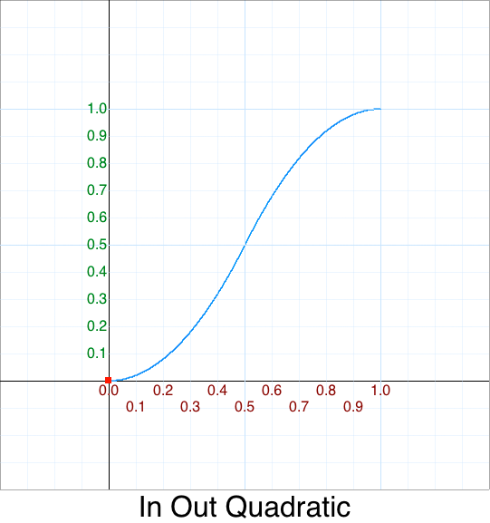
Cleanup - In

To avoid having to repeat myself there are some common idioms and expressions used in the original code:

Expression	Meaning	Replacement
x	not used	n/a
b	min x	0
c	max x	1
t/=d	elapsed time / duration	p

Note:

• Also keep in mind that we’ll drop the ease prefix so we can tell the difference between the original 5 parameter version and the optimized 1 parameter version.

With the fundamentals out of the way we can start optimizing all the easing functions.

Cleanup - In Back

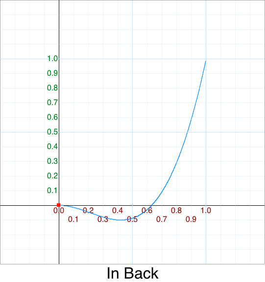
Original 5 argument version:

    easeInBack: function (x, t, b, c, d, s) {
        if (s == undefined) s = 1.70158;
        return c*(t/=d)*t*((s+1)*t - s) + b;
    },

Version 0 - rename easeInBack to InBack

Version 1 - remove x

    InBack: function (t, b, c, d, s) {
        if (s == undefined) s = 1.70158;
        return c*(t/=d)*t*((s+1)*t - s) + b;
    },

Version 2 - replace b = 0, c = 1

    InBack: function (t, d, s) {
        if (s == undefined) s = 1.70158;
        return 1*p*p*((s+1)*p - s) + 0;
    },

Version 3 - simplify t/=d = p

    InBack: function (p,s) {
        if (s == undefined) s = 1.70158;
        return p*p*((s+1)*p - s);
    },

Since most users will never override s with a custom constant it is safe to hard-code it; we’ll discuss this in a moment. The variable K is usually used to mean a constant – we’ll use that instead of s, the latter which is usually used to signal a scale factor.

Version 4 - Remove s

    InBack: function (p) {
        var K = 1.70158;
        return p*p*((K+1)*p - K);
    },

Version 5 - Reorder multiplication

    InBack: function (p) {
        var s = 1.70158;
        return p*p*(p*(s+1) - s);
    },

One-liner single argument version (1SAV):

    function InBack(p) { var k = 1.70158; return p*p*(p*(k+1) - k); }

The magic of 1.70158

If you are like me you might have an unanswered question:

• Where does the magic number 1.70158 come from?

Let’s graph various K values and overlay them using this legend:

K	Color
0	Red
1	Green
2	Blue

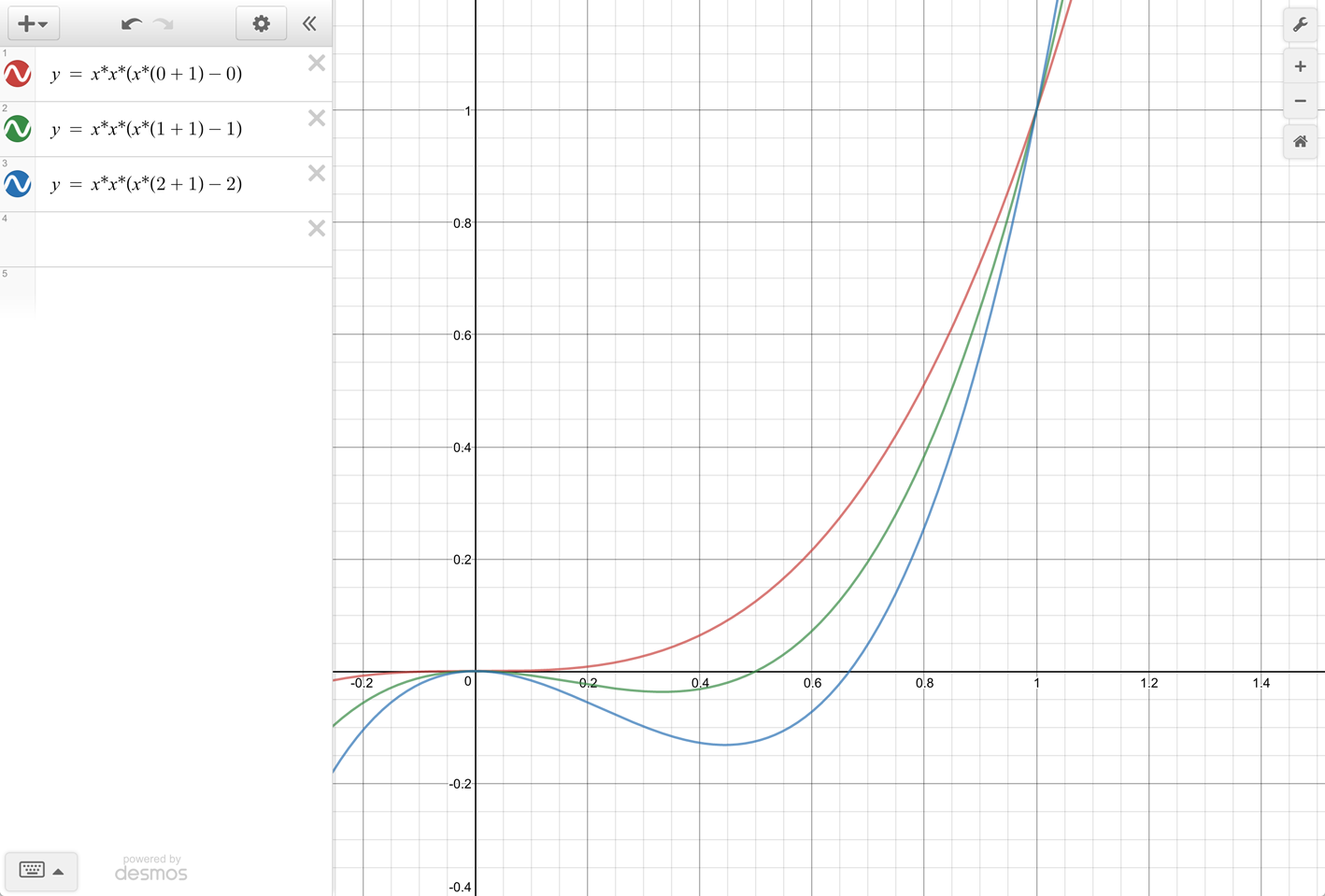
Hmm, K = 0 is exactly In Cubic.

   = p*p*(p*(K+1) - K)
   = p^3

Zooming into the K = 1.70158 graph:

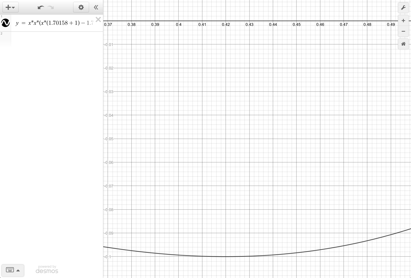
Hmm, it looks like this magic number was chosen to have a minimum of -10% !

Let’s confirm our hunch; it looks like y is -0.1 when x is around 0.42:

    f(x) = x*x*(x*(K+1) - K)
         = x*x*(x*(K+1) - K)
         = 0.42 * 0.42 * (0.42*(1.70158 + 1) - 1.70158)
         = -0.10000405296

So far so good. Can we get an exact value for x and for K ? We have one equation in two unknowns – we need two equations.

First, we need to expand this:

-0.1 = (K+1)*x^3 - K*x^2
   0 = K*x^3 + x^3 - K*x^2 + 0.1

We can’t solve this – yet. However, we actually have a 2nd equation.

Let’s use Calculus to find the x value of the minimum y = -0.1 value, that is, where the slope (or first derivate) is 0

Solving the differential equation:

    0 = d_dX f(x)
    0 = d_dX{ (K+1)*x^3 - K*x^2 }
    0 = d_dX{ K*x^3 + x^3 - K*x^2 }
    0 = 3*K*x^2 + 3*x^2 - 2*K*x
    0 = 3*K*x^2 - 2*K*x + 3*x^2
    0 = 3*K*x^2 - 2*K*x + 3*x^2

We can either solve for K:

    3*K*x^2 - 2*K*x = -3*x^2
    K*(3*x^2 - 2*x) = -3*x^2
    K = -3*x^2 / (3*x^2 - 2*x)

Or solve for x:

    0.1 = x^2*[ 3*K + 3 ] - 2*K*x
    2*K*x = x^2*[ 3*K + 3 ]
    2*K = x * (3*k + 3)
    x = 2*K / (3*K + 3)

Substituting the 2nd form back into the original equation leaves this polynomial::

    -0.1 = (K+1)*(2*K / (3*K + 3))^3 - K*(2*K / (3*K + 3))^2
    -0.1 = (K+1)*8*K^3 / (3*K + 3)^3 - 4*K^3 / (3*K + 3)^2
    -0.1*(3*K + 3)^3 = (K+1)*8*K^3 - 4*K^3*(3*K + 3)
    -0.1*27*(K+1)^3 = -4*K^4 - 4*K^3
    -0.1*(27*K^3 + 81*x^2 + 81*x + 27) = -4*K^4 - 4*K^3
    4*K^4 + 4*K^3 - 0.1*(27*K^3 + 81*K^2 + 81*K + 27) = 0
    4*K^4 + (4*K^3 - 2.7*K^3) - 8.1*K^2 - 8.1*K - 2.7 = 0
    4*K^4 + 1.3*K^3 - 8.1*K^2 - 8.1*K - 2.7 = 0

The graph of this equation looks like this:

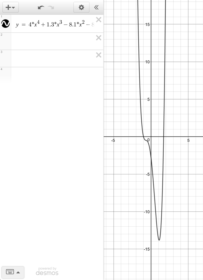FIXME

To solve this polynomial equation of degree 4, use your favorite symbolic calculator, such as GNU Octave. Don’t worry if you’re not familiar with GNU Octave, here are the 2 links that we need:

• Output Precision
• Finding Roots

Here are the GNU Octave commands to find the roots:

    format long;
    c = [ 4, 1.3, -8.1, -8.1, -2.7 ];
    roots ( c )

The 4 roots are:

Root	Real	Imaginary
1	+1.701540198866824	n/a
2	-1.0	n/a
3	-0.513270099433411	+0.365038654326168i
4	-0.513270099433411	-0.365038654326168i

We are only interested in the first root.

Why?

• Solving for x with K = -1 is a division by zero; this omits the 2nd root.
• We are not interested in the complex numbers so that rules out roots 3 and 4.

And solving for x with K = 1.701540198866824:

    x = 2*K / (3*K + 3)
    x = 2*1.701540198866824 / (3*1.701540198866824 + 3)
    x = 0.419893856494786

Produces this y value:

    = (K+1)*x^3 - K*x^2
    = (1.701540198866824 + 1)*0.419893856494786^3 - 1.701540198866824*0.419893856494786^2
    = -0.100000000000000

Pretty conclusive proof that value of K = 1.70158 was chosen to have -10% back.

“And now you know the rest of the story.” – Paul Harvey

Cleanup - In Bounce

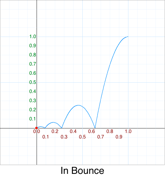
Original 5 argument version:

    easeInBounce: function (x, t, b, c, d) {
        return c - easeOutBounce (x, d-t, 0, c, d) + b;
    },

Hmm, it chains to easeOutBounce which has this prototype:

    easeOutBounce: function (x, t, b, c, d)

Since our cleaned upOutBounce() will eventually operate on the normalized input range [0,1] then, technically, we don’t need to know the internal details – just as long as we keep track of what is being passed in.

Version 1 - remove x

    InBounce: function (t, b, c, d) {
        return c - OutBounce (d-t, 0, c, d) + b;
    },

Version 2 - replace b = 0 and c = 1

    InBounce: function (t, d) {
        return 1 - OutBounce (d-t, 0, 1, d) + 0;
    },

Version 3 - remove extra OutBounce() arguments

    InBounce: function (t, d) {
        return 1 - OutBounce ( d-t, d);
    },

Normally p = t /d, but we have d-t / d. What is this equal to? With a little bit of algebra this simplies to:

    = (d - t)/d
    = d/d - t/d
    = 1 - p

Version 4 - simplify (d-t, d)

    InBounce: function ( p ) {
        return 1 - OutBounce ( 1-p );
    },

WOW - so much clearer. From our previous discussion of flips it should be immediately obvious that:

• InBounce = OutBounce flipped x, and flipped y !

This is a perfect example of why simplifying is so important. The whole point of Mathematics is to communicate efficiently. When you clutter up formulas with extra crap it becomes extremely difficult to see the forest from the trees.

One-liner single argument version (1SAV):

    function InBounce(p) { return 1 - OutBounce( 1-p ); }

Cleanup - In Circle

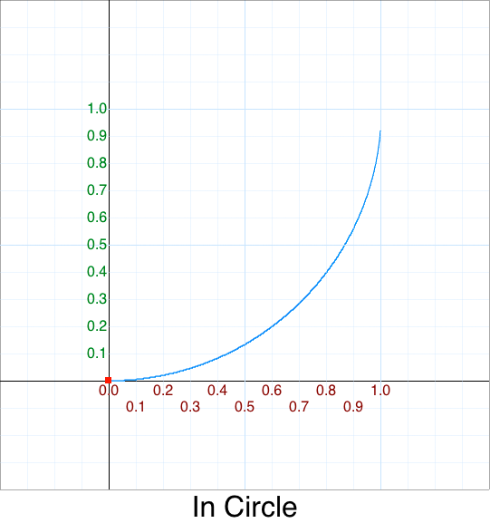
Original 5 argument version:

    easeInCirc: function (x, t, b, c, d) {
        return -c * (Math.sqrt(1 - (t/=d)*t) - 1) + b;
    },

Technically this easing should be called QuarterCircle but that deviates too much from the de facto name Circ.

Version 0 - Don’t abbreviate Circle

    InCircle: function (x, t, b, c, d) {
        return -c * (Math.sqrt(1 - (t/=d)*t) - 1) + b;
    },

Version 1 - remove x

    InCircle: function (t, b, c, d) {
        return -c * (Math.sqrt(1 - (t/=d)*t) - 1) + b;
    },

Version 2 - replace b = 0, c = 1

    InCircle: function (t, d) {
        return -1 * (Math.sqrt(1 - (t/=d)*t) - 1) + 0;
    },

Version 3 - simplify t/=d = p

    InCircle: function (t, d) {
        return -1 * (Math.sqrt(1 - p*p) - 1);
    },

Version 4 - distribute -1

    InCircle: function (t, d) {
        return -Math.sqrt(1 - p*p) + 1;
    },

Version 5 - rearrange terms

    InCircle: function (p) {
        return 1 - Math.sqrt(1 - p*p);
    },

One-liner single argument version (1SAV):

    InCircle: function (p) { return 1 - Math.sqrt(1 - p*p); },

Cleanup - In Cubic

Original 5 argument version:

    easeInCubic: function (x, t, b, c, d) {
        return c*(t/=d)*t*t + b;
    },

Version 0 - drop ease from name

Version 1 - remove x

    InCubic: function (t, b, c, d) {
        return c*(t/=d)*t*t + b;
    },

Version 2 - replace b = 0, c = 1

    InCubic: function (t, d) {
        return 1*(t/=d)*t*t + 0;
    },

Version 3 - simplify t/=d = p

    InCubic: function (p) {
        return p*p*p;
    },

One-liner single argument version (1SAV):

function InCubic(p) { return p*p*p; },

Cleanup - In Elastic

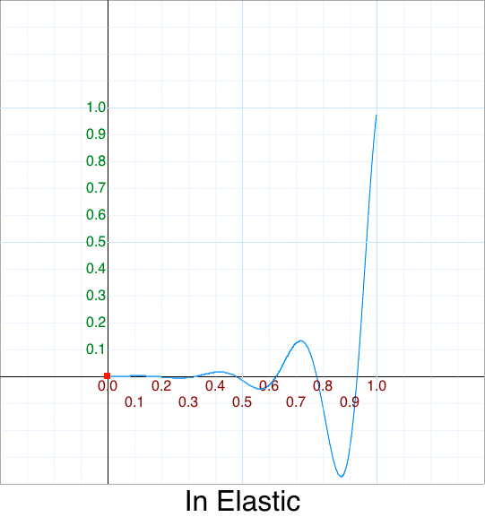
Original 5 argument version:

    easeInElastic: function (x, t, b, c, d) {
        var s=1.70158;var p=0;var a=c;
        if (t==0) return b;  if ((t/=d)==1) return b+c;  if (!p) p=d*.3;
        if (a < Math.abs(c)) { a=c; var s=p/4; }
        else var s = p/(2*Math.PI) * Math.asin (c/a);
        return -(a*Math.pow(2,10*(t-=1)) * Math.sin( (t*d-s)*(2*Math.PI)/p )) + b;
    },

UGH.

Version 0 - drop ease from name

Version 1 - Add line breaks

    InElastic: function (x, t, b, c, d) {
        var s=1.70158;
        var p=0;
        var a=c;

        if (t==0)
            return b;
        if ((t/=d)==1)
            return b+c;

        if (!p)
            p=d*.3;

        if (a < Math.abs(c)) {
            a=c;
            var s=p/4;
        }
        else
            var s = p/(2*Math.PI) * Math.asin (c/a);

        return -(a*Math.pow(2,10*(t-=1)) * Math.sin( (t*d-s)*(2*Math.PI)/p )) + b;
    },

Version 2 - Add whitespace

    InElastic: function (x, t, b, c, d) {
        var s = 1.70158;
        var p = 0;
        var a = c;

        if( t == 0 )
            return b;
        if( (t/=d) == 1)
            return b+c;

        if( !p )
            p = d*.3;

        if( a < Math.abs(c) ) {
                a = c;
            var s = p/4;
        }
        else
            var s = p/(2*Math.PI) * Math.asin (c/a);

        return -(a*Math.pow(2,10*(t-=1)) * Math.sin( (t*d-s)*(2*Math.PI)/p )) + b;
    },

Version 3 - Static Analysis & Dynamic Analysis

    InElastic: function (x, t, b, c, d) {
        var s = 1.70158; // useless constant -- not used as it is over-written
        var p = 0;
        var a = c;

        if( t == 0 )
            return b;
        if( (t/=d) == 1 )
            return b+c;

        if( !p ) // useless conditional -- always true
            p = d*.3;

        // Over-engineered if
        // a=c; if (a < Math.abs(c)) == if (c < Math.abs(c)) == if( c < 0 )
        if( a < Math.abs(c) ) { // uncommon case: if( c < 0)
            a=c;         // why?? redundant
            var s = p/4; // s has same value in both true and false clauses
        }
        else // common case: if (c >= 0)
            var s = p/(2*Math.PI) * Math.asin (c/a);  // Over-engineered: s=p/4;
            // c/a == +1  Math.asin(+1) = +90 deg
            // c/a == -1  Math.asin(-1) = -90 deg
            // but a=c, and if(c<0) then ... else c>0, therefore c/a always +1
            // var s = p/(2*Math.PI) * Math.asin(1);

            // PI/2 radians =  90 degrees
            // 2 PI radians = 360 degrees
            // var s = p/(2*Math.PI) * Math.PI/2;
            // var s = p/4;

        // unnecessary a, since a=c
        return -(a*Math.pow(2,10*(t-=1)) * Math.sin( (t*d-s)*(2*Math.PI)/p )) + b;
    },

Version 4 - Remove redundant code

    InElastic: function (x, t, b, c, d) {
        var p = d*.3;
        var s = p/4; // 4 bounces

        if (t < 0)
            return b;

        t /= d;
        if (t > 1)
            return b+c;

        t -= 1;
        return -(c*Math.pow(2,10*t) * Math.sin( (t*d-s)*(2*Math.PI)/p )) + b;
    },

Version 5 - Robustness: Handle edge cases

    InElastic: function (x, t, b, c, d) {
        var p = d*.3;
        var s = p/4;

        if (d <= 0) // clamp position
            return b; // b -> 0.0

        if (t <= 0) // clamp position
            return b; // b -> 0.0

        t /= d;
        if (t >= 1) // clamp position
            return b+c; // b+c -> 1.0

        t -= 1;
        return -(c*Math.pow(2,10*t) * Math.sin( (t*d-s)*(2*Math.PI)/p )) + b;
    },

Version 6 - Refactor last term sin( .. )

    = (t*d-s)*(2*Math.PI)/p
    = (t*d-p/4)   *(2*Math.PI)/p
    = (t*d-d*.3/4)*(2*Math.PI)/(d*.3)
    = d*(t-.3/4)  *(2*Math.PI)/(d*.3)
    = (t-.3/4)    *(2*Math.PI)/.3
    = (t/.3-1/4)  *(2*Math.PI)
    = (2*t/.3-1/2)*   Math.PI
    = (40*t-3)    *   Math.PI/6

Note:

• 40/6
• = 6.666…
• = 2/0.3
• = 1/0.3 * 2 * …PI…

That is:

    return -(c*Math.pow(2,10*t) * Math.sin( (t*d-s)     *(2*Math.PI)/k      )) + b; // original
    return -(c*Math.pow(2,10*t) * Math.sin( (t*d-k/4)   *(2*Math.PI)/k      )) + b;
    return -(c*Math.pow(2,10*t) * Math.sin( (t*d-d*.3/4)*(2*Math.PI)/(d*.3) )) + b;
    return -(c*Math.pow(2,10*t) * Math.sin( d*(t-.3/4)  *(2*Math.PI)/(d*.3) )) + b;
    return -(c*Math.pow(2,10*t) * Math.sin( (t-.3/4)    *(2*Math.PI)/.3     )) + b; // can factor out duration
    return -(c*Math.pow(2,10*t) * Math.sin( (t/.3-1/4)  *(2*Math.PI)        )) + b;
    return -(c*Math.pow(2,10*t) * Math.sin( (2*t/.3-1/2)*   Math.PI         )) + b;
    return -(c*Math.pow(2,10*t) * Math.sin( (40*t-3)    *   Math.PI/6       )) + b; // simplified

Version 7 - Simplified & Optimized original style ‘easeInElastic’

    easeInElastic: function (x, t, b, c, d) {
        if (t <= 0) return b  ;
        if (t >= d) return b+c;
        t /= d;
        t -= 1;
        return -(c*Math.pow(2,10*t) * Math.sin( (40*t-3) * Math.PI/6 )) + b;
    },

Version 8 - remove x

    InElastic: function (t, b, c, d) {
        t /= d;
        if (t <= 0) return b  ;
        if (t >= 1) return b+c;
        t -= 1;
        return -(c*Math.pow(2,10*t) * Math.sin( (40*t-3) * Math.PI/6 )) + b;
    },

Version 9 - replace b = 0, c = 1

    InElastic: function (t, d) {
        t /= d;
        if (t <= 0) return 0  ;
        if (t >= 1) return 0+1;
        t -= 1;
        return -(1*Math.pow(2,10*t) * Math.sin( (40*t-3) * Math.PI/6 )) + 0;
    },

Version 10 - simplify t/=d = p

    InElastic: function (p) {
        if (p <= 0) return 0;
        if (t >= 1) return 1;
        t -= 1;
        return -(Math.pow(2,10*t) * Math.sin( (40*t-3) * Math.PI/6 ));
    },

Whew! We can now finally provide the single argument version using m = p-1:

    InElastic: function(p) {
        var m = p-1;
        if (p <= 0) return 0;
        if (p >= 1) return 1;
        return -Math.pow( 2, 10*m ) * Math.sin( (40*m-3) * Math.PI/6 );
    },

There are some variations, depending on how much inlining of terms you want to do:

• With m removed, replaced with p-1:

    easeInElastic: function(p) {
        return -Math.pow( 2,10*(p-1) ) * Math.sin( ((p-1)*40 - 3) * Math.PI/6 );
    },

• With -1 optimized out:

    InElastic: function(p) {
        return -  Math.pow( 2,10*p-10 ) * Math.sin( (40*p-43) * Math.PI/6 ); // m=p-1, m*40-1 -> (p-1)*40-3 -> 40*p-43
    },

NOTE: jQuery UI does NOT match the original as their constants are incorrect

Cleanup - In Exponent 2

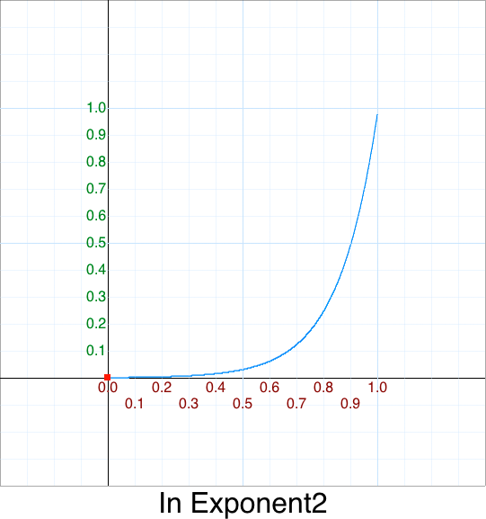
Original 5 argument version:

    easeInExpo: function (x, t, b, c, d) {
        return (t==0) ? b : c * Math.pow(2, 10 * (t/d - 1)) + b;
    },

Version 0 - drop ease from name; rename Expo to Exponent2

    InExponent2: function (x, t, b, c, d) {
        return (t==0) ? b : c * Math.pow(2, 10 * (t/d - 1)) + b;
    },

Version 1 - remove x

    InExponent2: function (t, b, c, d) {
        return (t==0) ? b : c * Math.pow(2, 10 * (t/d - 1)) + b;
    },

Version 2 - semantically uncompress out-of-bounds

    InExponent2: function (t, b, c, d) {
        if (t <= 0) return b;
        return c * Math.pow(2, 10 * (t/d - 1)) + b;
    },

Version 3 - replace b = 0, c = 1

    InExponent2: function (t, d) {
        if (t <= 0) return 0;
        return 1 * Math.pow(2, 10 * (t/d - 1)) + 0;
    },

Version 4 - simplify t/d = p

    InExponent2: function (p) {
        if (p <= 0) return 0;
        return Math.pow(2, 10 * (p-1));
    },

One-liner single argument version (1SAV):

    function InExponent2(p) { if (p <= 0) return 0; return Math.pow( 2, 10*(p-1) ); }

Cleanup - In Exponent e

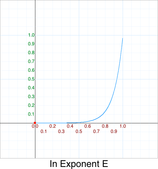
This is missing in the original since Exponent2 was abbreviated as Expo and there was, sadly, no need for completeness. Let’s fix this deficiency.

This is what a normal graph of e^x looks like:

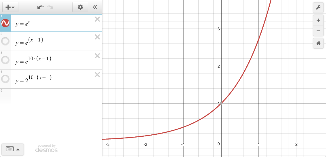
We can “shift” the y-intercept of the graph over to the right via: e^(x-#)

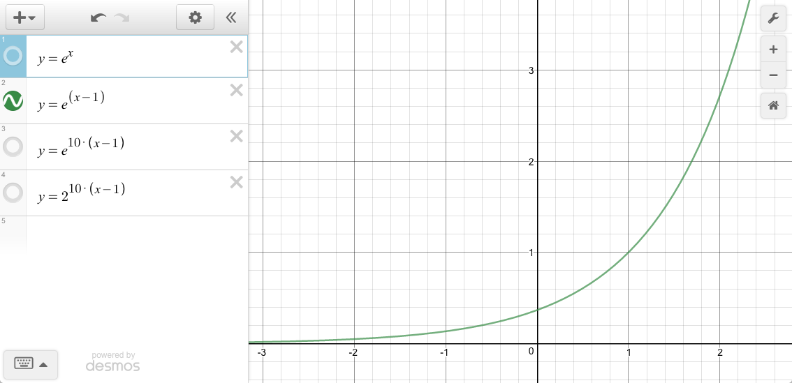
However, an In function starts at zero,and ends at one. We need to “compress” the width. We’ll match what Exponent2 does and use a scale value of 10.

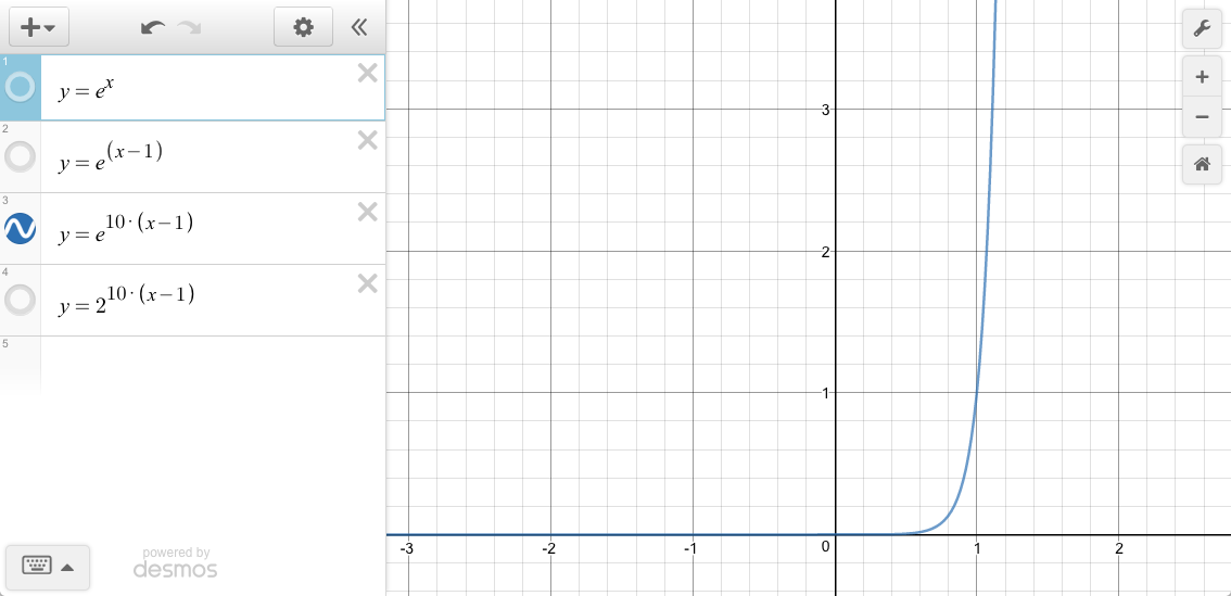
To see how Exponent2 and ExponentE compare:

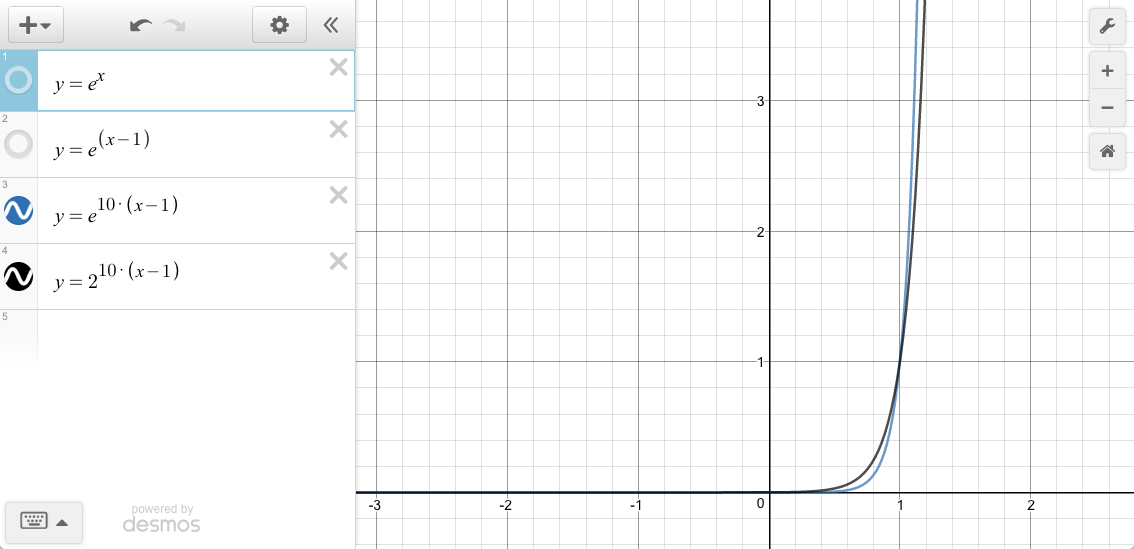
In the original style the easing function would look like this:

    easeInExponentE: function (x, t, b, c, d) {
        return (t==0) ? b : c * Math.pow( Math.E, 10 * (t/d - 1)) + b;
    },

Version 0 - drop ease from name

Version 1 - remove x

    InExponentE: function (t, b, c, d) {
        return (t==0) ? b : c * Math.pow( Math.E, 10 * (t/d - 1)) + b;
    },

Version 2 - replace b = 0, c = 1

    InExponentE: function (t, d) {
        return (t==0) ? 0 : 1 * Math.pow( Math.E, 10 * (t/d - 1)) + 0;
    },

Version 3 - uncompress edge condition

    InExponentE: function (t, d) {
        if (t <= 0) return 0;
        reutrn Math.pow( Math.E, 10 * (t/d - 1));
    },

Version 4 - simplify t/d = p

    InExponentE: function (p) {
        if (p <= 0) return 0;
        return Math.pow( Math.E, 10 * (p - 1));
    },

One-liner single argument version (1SAV):

    function InExponentE(p) { if (p <= 0) return 0; return Math.pow( Math.E, 10*(p-1) ); },

Cleanup - In Log10

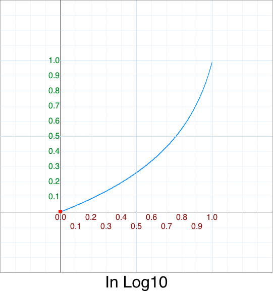
This is also missing in the original. Let’s add it for completeness.

Here is a graph of Log10(x):

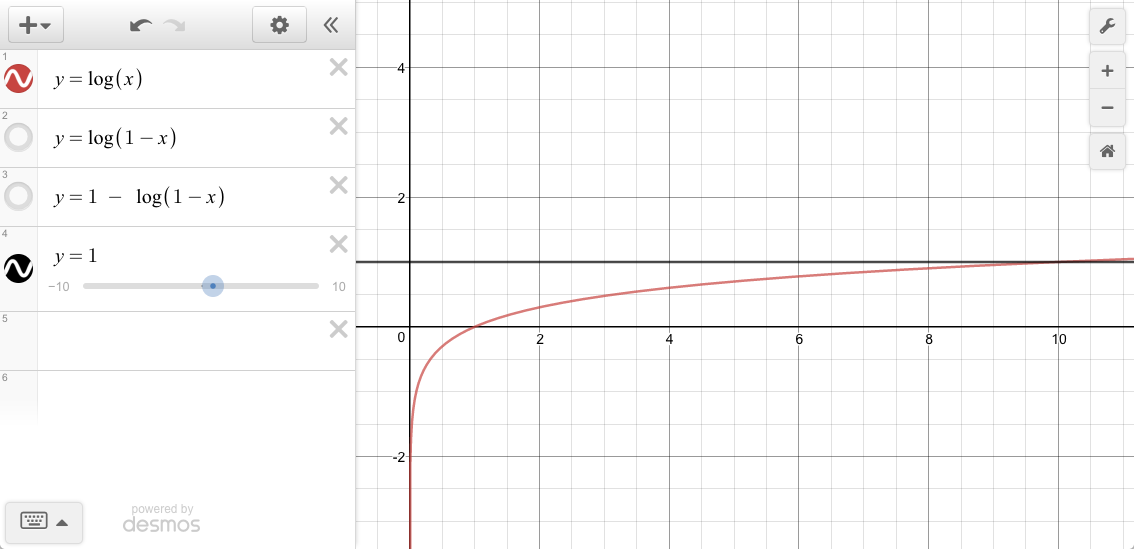
We’re interested in the range { 1 <= x <= 10 }

x	y = log10(x)
1	0
10	1

Since input p ranges from 0 to 1 we need to re-map it:

p	x	y = log10(x)
0	1	0
1	10	1

    var x = (p*9)+1
    return Math.log10( x );

But notice this shape is an Out shape, not an In shape.

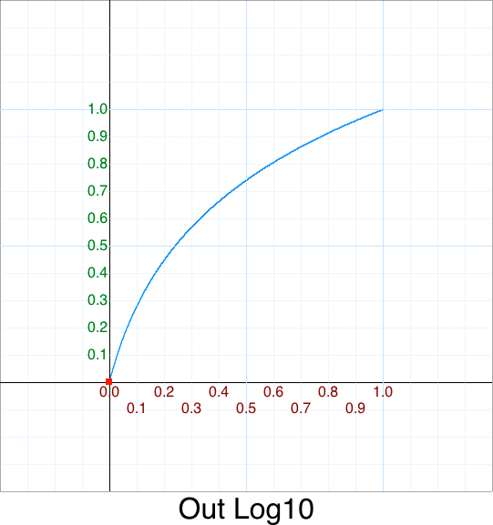
We’ll defer the rest of this explanation by having In = Out flipped x and flipped y.

    function InLog10(p) { return 1 - OutLog10( 1-p ); }

Cleanup - In Octic

This is missing in the original but it is trivial to add:

    easeInOctic: function (x, t, b, c, d) {
        return c*(t/=d)*t*t*t*t*t*t*t + b;;
    },

Version 0 - drop ease from name

One-liner single argument version (1SAV):

    function InOctic(p) { return p*p*p*p*p*p*p*p; },

Cleanup - In Quadratic

We already covered this above and know the answer should be p*p but the extra practice doesn’t hurt.

    easeInQuad: function (x, t, b, c, d) {
        return c*(t/=d)*t + b;
    },

Version 0 - drop ease from name; unabbreviate Quad for clarity

    InQuadratic: function (x, t, b, c, d) {
        return c*(t/=d)*t + b;
    },

Version 1 - remove x

    InQuadratic: function (t, b, c, d) {
        return c*(t/=d)*t + b;
    },

Version 2 - replace b = 0, c = 1

    InQuadratic: function (t, d) {
        return 1*(t/=d)*t + 0;
    },

Version 3 - simplify t/=d = p

    InQuadratic: function (p) {
        return p*p;
    },

One-liner single argument version (1SAV):

    function InQuadratic(p) { return p*p; },

Cleanup - In Quartic

Original 5 argument version:

    easeInQuart: function (x, t, b, c, d) {
        return c*(t/=d)*t*t*t + b;
    },

Version 0 - drop ease from name; unabbreviate Quart for clarity

    InQuart: function (x, t, b, c, d) {
        return c*(t/=d)*t*t*t + b;
    },

Version 1 - remove x

    InQuart: function (t, b, c, d) {
        return c*(t/=d)*t*t*t + b;
    },

Version 2 - replace b = 0, c = 1

    InQuart: function (t, d) {
        return 1*(t/=d)*t*t*t + 0;
    },

Version 3 - simplify t/=d = p

    InQuart: function (p) {
        return p*p*p*p;
    },

One-liner single argument version (1SAV):

    function InQuartic(p) { return p*p*p*p; },

Cleanup - In Quintic

Original 5 argument version:

    easeInQuint: function (x, t, b, c, d) {
        return c*(t/=d)*t*t*t*t + b;
    },

Version 0 - drop ease from name; unabbreviate Quint for clarity

    InQuintic: function (x, t, b, c, d) {
        return c*(t/=d)*t*t*t*t + b;
    },

Version 1 - remove x

    InQuintic: function (t, b, c, d) {
        return c*(t/=d)*t*t*t*t + b;
    },

Version 2 - replace b = 0, c = 1

    InQuintic: function (t, d) {
        return 1*(t/=d)*t*t*t*t + 0;
    },

Version 3 - simplify t/=d = p

    InQuintic: function ( p ) {
        return p*p*p*p*p;
    },

One-liner single argument version (1SAV):

    function InQuintic(p) { return p*p*p*p*p; },

Cleanup - In Septic

Polynomials above degree 5 are missing in the original. Let’s add degree 7, Septic, for completeness.

In the original style it would be written as:

    easeInSept: function (x, t, b, c, d) {
        return c*(t/=d)*t*t*t*t*t*t + b;
    },

Version 0 - drop ease from name; unabbreviate Sept for clarity

It is easy to verify we have the correct numbers of terms above. There should be n-1 terms of t.

One-liner single argument version (1SAV):

    function InSeptic(p) { return p*p*p*p*p*p*p; },

For the 1-liner there should be 7 terms of p.

Cleanup - In Sextic

Polynomials above degree 5 are missing in the original. Let’s add degree 6 for completeness.

    easeInSext: function (x, t, b, c, d) {
        return c*(t/=d)*t*t*t*t*t + b;
    },

Version 0 - drop ease from name; unabbreviate Sext for clarity

One-liner single argument version (1SAV):

    function InSextix(p) { return p*p*p*p*p*p; },

For the 1-liner there should be 6 terms of p.

Cleanup - In Sine

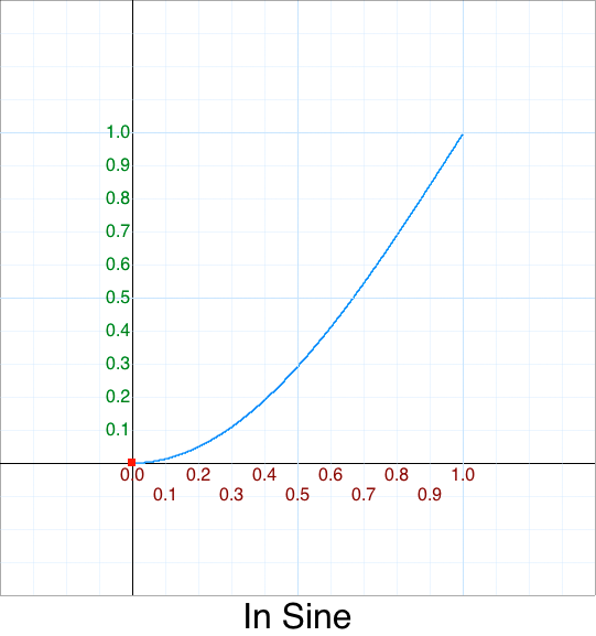
Original 5 argument version:

    easeInSine: function (x, t, b, c, d) {
        return -c * Math.cos(t/d * (Math.PI/2)) + c + b;
    },

There are 2 inconsistencies with this:

• It is called Sine even though it uses Cosine – there is a reason for this but it will have to wait for OutSine
• It should have been abbreviated Sin

We’ll ignore renaming this to InCos so as not to confuse people for why we have a InCos but not an InSine like everyone else. “Sometimes a consistent, bad standard is better then an inconsistent, good standard.”

Sometimes. :-/

Moving on, the graph of cos(x) looks like this:

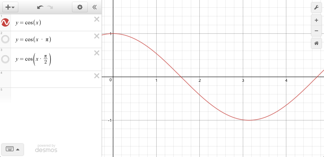
But our input p is between 0 and 1:

p	x	y
0	0	1
1	?	0

We need to scale our input p such that x is in-between 0 and π (inclusive.)

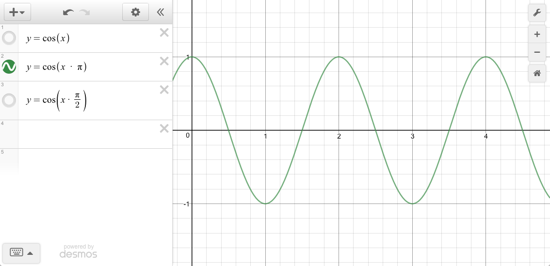
But we’ve compressed the x too much. When p = 1 we need y = 0 in our equation cos(x * pi/n) = 0. Solving for n when x = 1:

    cos( x * pi/n) = 0
    acos( cos( x * pi/n ) ) = acos( 0 )
    1 * 180_degrees / n = 90_degrees
    180_degrees / 90_degrees = n

… leaves 2.

    var x = p/2
    y = cos( x * PI );

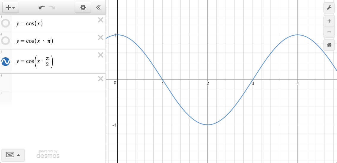
Version 0 - drop ease from name

Version 1 - remove x

    InSine: function (t, b, c, d) {
        return -c * Math.cos(t/d * (Math.PI/2)) + c + b;
    },

Version 2 - replace b = 0, c = 1

    InSine: function (t, d) {
        return -1 * Math.cos(t/d * (Math.PI/2)) + 1 + 0;
    },

Version 3 - simply

    InSine: function (t, d) {
        return 1 - Math.cos(t/d * (Math.PI/2));
    },

Version 4 - simplify t/d = p

    InSine: function (p) {
        return 1 - Math.cos(p * (Math.PI/2));
    },

Version 5 - replace slow division with multiplication

    InSine: function (p) {
        return 1 - Math.cos( p * Math.PI * 0.5 );
    },

One-liner single argument version (1SAV):

    function InSine(p) { return 1 - Math.cos( p * Math.PI*0.5 ); }

Cleanup - In Square Root

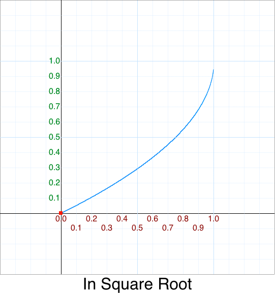
Again, there isn’t one so we’ll add one for completeness.

Like In Bounce, for InSquareRoot we defer to OutSquareRoot:

• InSquareRoot = OutSquareRoot flipped x, and flipped y

In the original style:

    easeInSqrt: function (x, t, b, c, d) {
        return c - easeOutSqrt( x, d-t, 0, c, d ) + b;
    },

Version 0 - drop ease from name

One-liner single argument version (1SAV):

    function InSquareRoot(p) { return 1 - OutSquareRoot( 1-p ); }

Cleanup - Out

Cleanup - Out Back

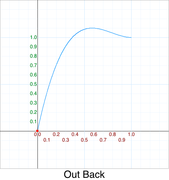
Original 5 argument version:

    easeOutBack: function (x, t, b, c, d, s) {
        if (s == undefined) s = 1.70158;
        return c*((t=t/d-1)*t*((s+1)*t + s) + 1) + b;
    },

Version 0 - drop ease from name

Version 1 - Remove x

    OutBack: function (t, b, c, d, s) {
        if (s == undefined) s = 1.70158;
        return c*((t=t/d-1)*t*((s+1)*t + s) + 1) + b;
    },

Version 2 - Replace b = 0, c = 1

    OutBack: function (t,d, s) {
        if (s == undefined) s = 1.70158;
        return 1*((t=t/d-1)*t*((s+1)*t + s) + 1) + 0;
    },

Version 3 - replace t/d with p

    OutBack: function (p, s) {
        if (s == undefined) s = 1.70158;
        return (p-1)*(p-1)*((s+1)*(p-1) + s) + 1;
    },

Version 4 - Factor p-1 with m

    OutBack: function (p, s) {
        if (s == undefined) s = 1.70158;
        var m = p-1;
        return m*m*((s+1)*m + s) + 1;
    },

Version 5 - Re-order m and + 1

    OutBack: function (p, s) {
        if (s == undefined) s = 1.70158;
        var m = p-1;
        return 1 + m*m*(m*(s+1) + s);
    },

Version 6 - Make 1.70158 constant K

    OutBack: function (p) {
        var K = 1.70158;
        return 1 + m*m*(m*(k+1) + k);
    },

One-liner single argument version (1SAV):

    function OutBack(p) { var m=p-1, K = 1.70158; return 1 + m*m*(m*(K+1) + K); }

Cleanup - Out Bounce

Cleanup - Out Circle

Cleanup - Out Cubic

Cleanup - Out Elastic

If we are lazy …

• Reverse x via (1-p), and
• Flip y via 1 - f(x)

leaves us with:

    OutElastic: function(p) { return 1 - this.easeInElastic( 1-p ); },

However that isn’t optimal:

With manual substitution:

One-liner single argument version (1SAV):

    OutElastic: function(p) { return 1+(Math.pow( 2,10*-p ) * Math.sin( (-p*40 - 3) * Math.PI/6 )); },

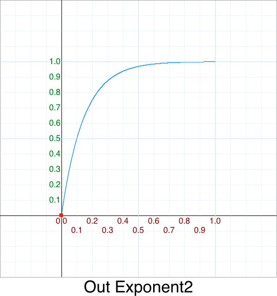
Cleanup - Out Exponent 2

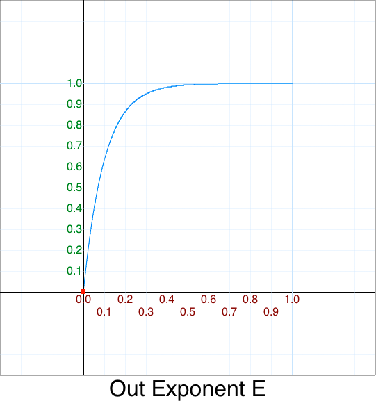
Cleanup - Out Exponent e

Cleanup - Out Log10

Cleanup - Out Octic

Cleanup - Out Quadratic

Original 5 argument version:

    easeOutQuad: function (x, t, b, c, d) {
        return -c*(t/=d)*(t-2) + b;
    },

Version 0 - rename Quad to Quadratic

    OutQuadratic: function (x, t, b, c, d) {
        return -c*(t/=d)*(t-2) + b;
    },

Version 1 - remove x

    OutQuadratic: function (t, b, c, d) {
        return -c*(t/=d)*(t-2) + b;
    },

Version 2 - replace b = 0, c = 1

    OutQuadratic: function (t, d) {
        return -1*(t/=d)*(t-2) + 0;
    },

Version 3 - simplify t/=d = p

    OutQuadratic: function (p) {
        return -1*(p)*(p-2);
    },

Version 4 - simplify

    OutQuadratic: function (p) {
        return -p*(p-2);
    },

Version 5 - factor out p-1

Why p-1 ? To show the symmetry of the Out power series.

    = -1*p*(p-2)
    = -p*(p-2)
    = -p^2+2p
    = 1-(p^2+2p-1)
    = 1-((p-1)*(p-1))

Leaving:

    OutQuadratic: function (p) {
        var m = p-1;
        return 1-(m*m);
    },

One-liner single argument version (1SAV):

    function OutQuadratic(p) { var m=p-1; return 1-m*m; },

Cleanup - Out Quartic

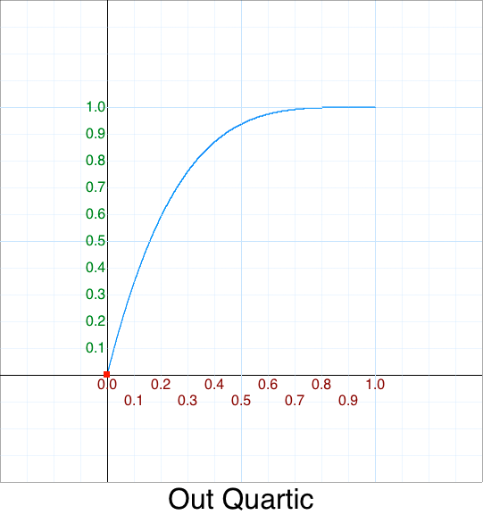
Original 5 argument version:

    easeOutQuart: function (x, t, b, c, d) {
        return -c * ((t=t/d-1)*t*t*t - 1) + b;
    },

Version 0 - unabbreviate Quart

    OutQuartic: function (x, t, b, c, d) {
        return -c * ((t=t/d-1)*t*t*t - 1) + b;
    },

Version 1 - remove x

    OutQuartic: function (t, b, c, d) {
        return -c * ((t=t/d-1)*t*t*t - 1) + b;
    },

Version 2 - replace b = 0, c = 1

    OutQuartic: function (t, d) {
        return -1 * ((t=t/d-1)*t*t*t - 1) + 0;
    },

Version 3 - simplify t/=d = p

    OutQuartic: function (p) {
        var m = p - 1
        return -1 * (m*m*m*m - 1);
    },

Version 4 - distribute -1

    = -1 * (m*m*m*m - 1)
    = -m*m*m*m + 1)
    = 1 - m*m*m*m

    OutQuartic: function (t, d) {
        var m = p-1;
        return 1 - m*m*m*m;
    },

One-liner single argument version (1SAV):

    function OutQuartic(p) { var m=p-1; return 1-m*m*m*m; }

Cleanup - Out Quintic

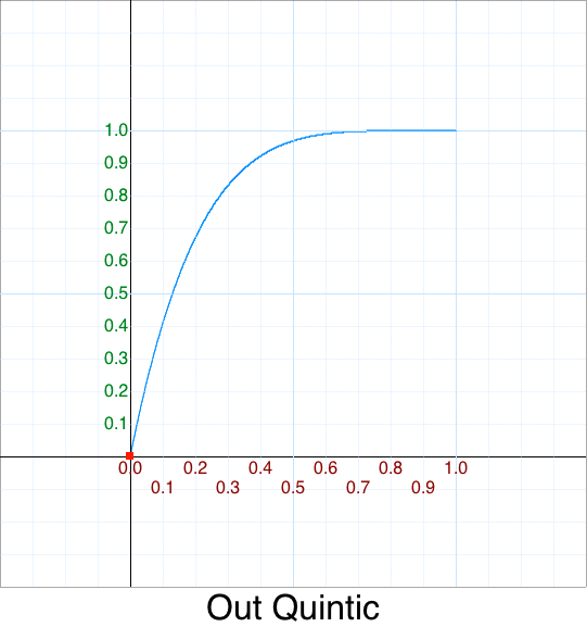
Cleanup - Out Septic

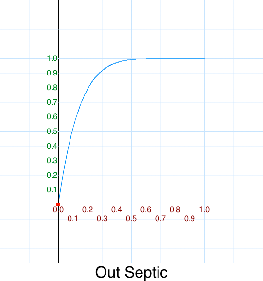
Cleanup - Out Sextic

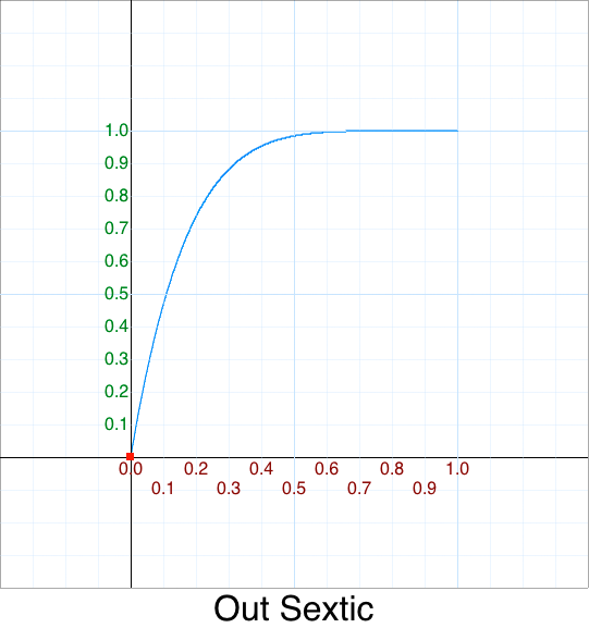
Cleanup - Out Sine

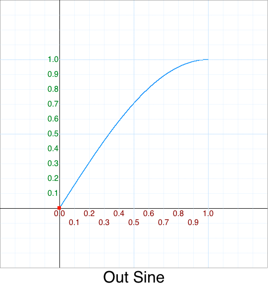
Cleanup - Out Square Root

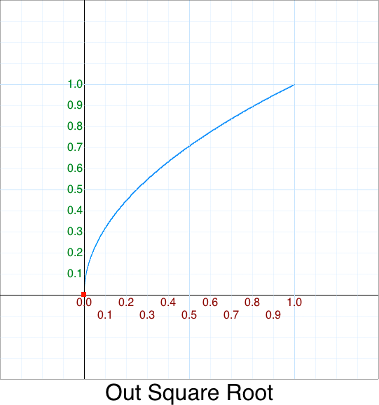
Cleanup In Out

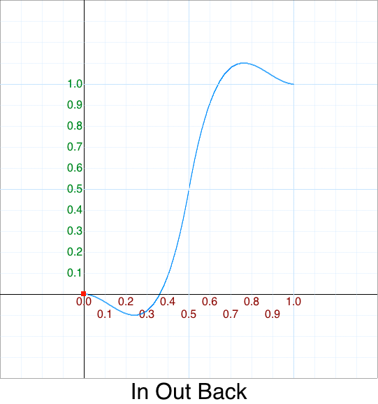
Cleanup - In Out Back

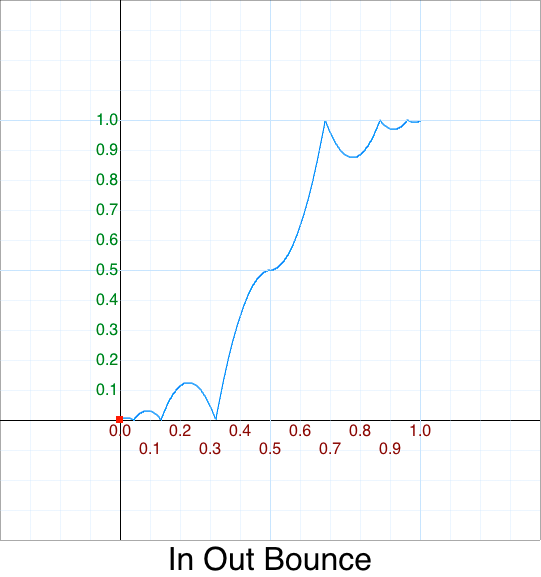
Cleanup - In Out Bounce

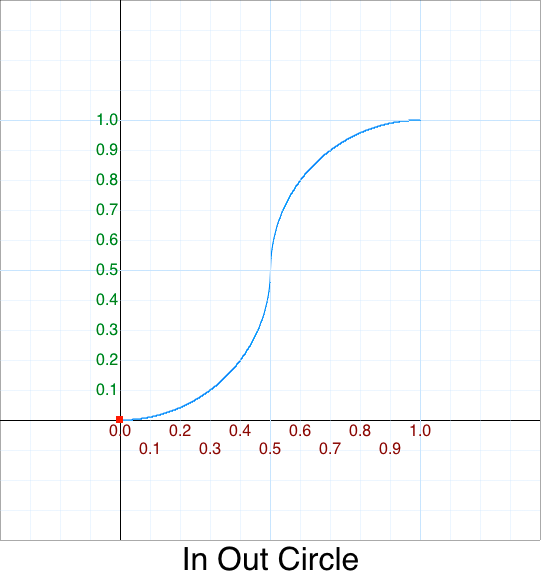
Cleanup - In Out Circle

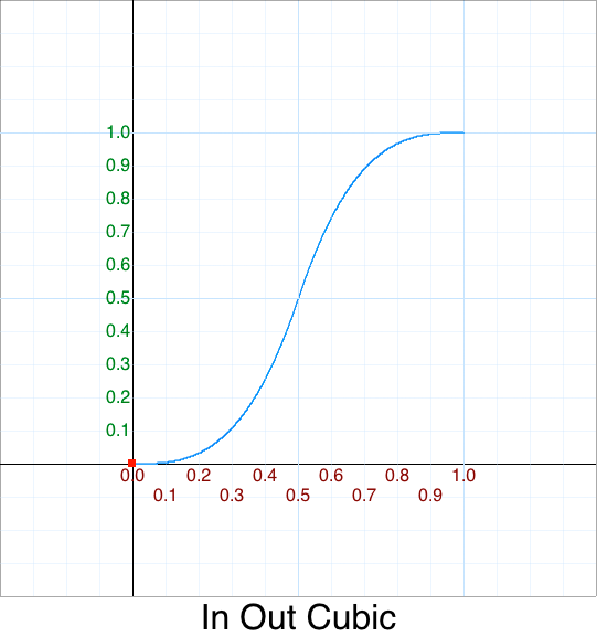
Cleanup - In Out Cubic

Cleanup - In Out Elastic

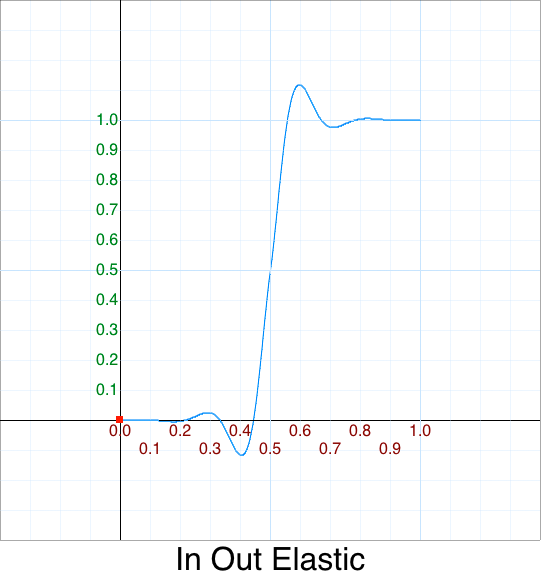
    easeInOutElastic: function(p) {
        if (p < 0.5) return     this.easeInElastic ( t     )*0.5;
        else         return 1 - this.easeOutElastic( t - 1 )*0.5;
    },

Cleanup - In Out Exponent 2

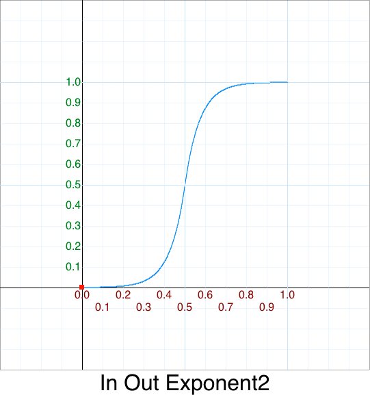
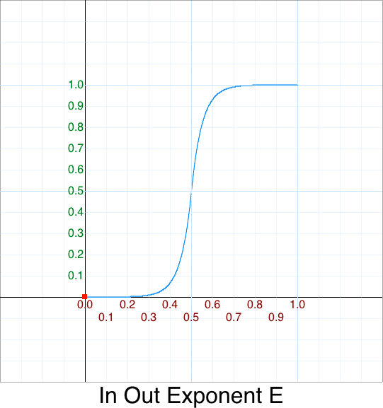
Cleanup - In Out Exponent e

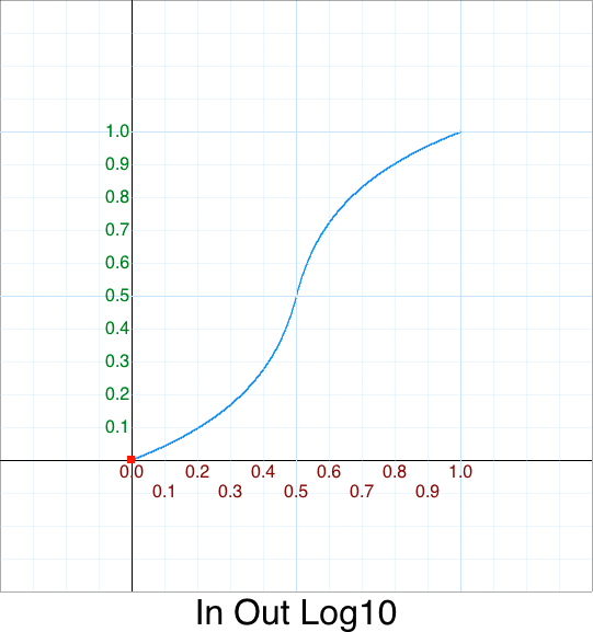
Cleanup - In Out Log10

Cleanup - In Out Octic

Cleanup - In Out Quadratic

Cleanup - In Out Quartic

Cleanup - In Out Quintic

Cleanup - In Out Septic

Cleanup - In Out Sextic

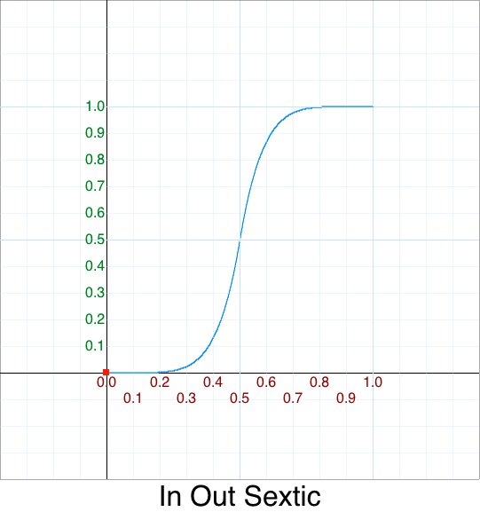
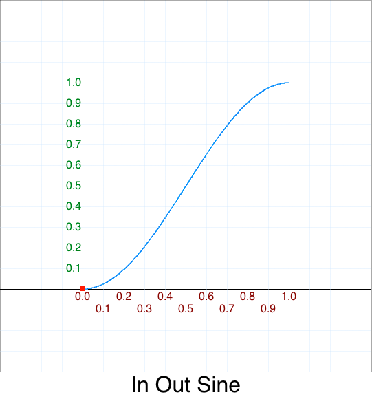
Cleanup - In Out Sine

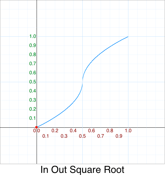
Cleanup - In Out Square Root

Verification

Any good scientist verifies the data. As computer scientists any time we do optimizations we need to as well – else we could be introducing bugs.

• “It doesn’t matter how fast you get the answer if it is wrong!”

This will be forthcoming.

The Art and Science of Beautiful Code

Let’s collect all the power functions we’ve cleaned up and stick them in an array for easy access.

First, we’ll need an enumeration – but since JS is so badly designed it doesn’t have one we’ll fake it using Javascript object notation syntax (JSON). This is just a fancy way of saying we’ll have an object with a named key,value pair.

Why JSON?

Because you don’t need to clutter up the code with more junk. e.g. You can see the over-engineering extremes some people go to just to work around a bad language and not using the native idioms.

var Easing = Object.freeze(
{
    NONE            :  0,
    LINEAR          :  1,

// Power
    IN_QUADRATIC    :  2,
    IN_CUBIC        :  3,
    IN_QUARTIC      :  4,
    IN_QUINTIC      :  5,
    IN_SEXTIC       :  6,
    IN_SEPTIC       :  7,
    IN_OCTIC        :  8,

    OUT_QUADRATIC   :  9,
    OUT_CUBIC       : 10,
    OUT_QUARTIC     : 11,
    OUT_QUINTIC     : 12,
    OUT_SEXTIC      : 13,
    OUT_SEPTIC      : 14,
    OUT_OCTIC       : 15,

    IN_OUT_QUADRATIC: 16,
    IN_OUT_CUBIC    : 17,
    IN_OUT_QUARTIC  : 18,
    IN_OUT_QUINTIC  : 19,
    IN_OUT_SEXTIC   : 20,
    IN_OUT_SEPTIC   : 21,
    IN_OUT_OCTIC    : 22,

// Standard
    // :

// Non-Standard
   // :
});

The reason for Easing.NONE is that we’ll use this as a placeholder to signal that an animation is not currently active in our animation loop. See Widget Line #488

True Beautify Lies on the Inside

Most inexperienced programmers would collate the functions like this.

    function None(p) { return 1; }
    function Linear(p) { return p; }
    function InQuadratic(p) { return p*p; }
    function InCubic(p) { return p*p; }
    function InQuartic(p) { return p*p*p*p; }
    function InQuintic(p) { return p*p*p*p*p; }
    function InSextic(p) { return p*p*p*p*p*p; }
    function InSeptic(p) { return p*p*p*p*p*p*p; }
    function InOctic(p) { return p*p*p*p*p*p*p*p; }

This is crap code.

Why?

• While Functionally it is correct,
• Visuallly it is code vomit.

You can’t easily tell if we made a mistake and accidently left off one of the p variables – which I intentionally did. Now before you go looking for it let’s reformat this code which will make your job trivial to find.

How do experienced programmers write beautiful code?

• use descriptive variables names
• use multi-column alignment and,
• use whitespace

We’ll also add comments on the end in case someone isn’t familiar with all the polynomial degree terminology.

    function None           (p) { return 1;               }, // p^0 Placeholder for no active animation
    function Linear         (p) { return p;               }, // p^1 Note: In = Out = InOut
    function InQuadratic    (p) { return p*p;             }, // p^2 = Math.pow(p,2)
    function InCubic        (p) { return p*p;             }, // p^3 = Math.pow(p,3)
    function InQuartic      (p) { return p*p*p*p;         }, // p^4 = Math.pow(p,4)
    function InQuintic      (p) { return p*p*p*p*p;       }, // p^5 = Math.pow(p,5)
    function InSextic       (p) { return p*p*p*p*p*p;     }, // p^6 = Math.pow(p,6)
    function InSeptic       (p) { return p*p*p*p*p*p*p;   }, // p^7 = Math.pow(p,7)
    function InOctic        (p) { return p*p*p*p*p*p*p*p; }, // p^8 = Math.pow(p,8)

It becomes trivial to spot that InCubic is missing a *p term and should be this:

    function InCubic        (p) { return p*p*p;           }, // p^3 = Math.pow(p,3)

Beauty on the Outside

Let’s do the same thing for Out

    function OutQuadratic(p) { var m=p-1; return 1-m*m; },
    function OutCubic(p) { var m=p-1; return 1+m*m*m; },
    function OutQuartic(p) { var m=p-1; return 1-m*m*m*m; },
    function OutQuintic(p) { var m=p-1; return 1+m*m*m*m*m; },
    function OutSextic(p) { var m=p-1; return 1-m*m*m*m*m*m; },
    function OutSeptic(p) { var m=p-1; return 1+m*m*m*m*m*m*m;},
    function OutOctic(p) { var m=p-1; return 1-m*m*m*m*m*m*m*m; },

The reason I factored p-1 is that when we use alignment we can see the beautiful symmetry of the Out Power functions:

    function OutQuadratic   (p) { var m=p-1; return 1-m*m;             },
    function OutCubic       (p) { var m=p-1; return 1+m*m*m;           },
    function OutQuartic     (p) { var m=p-1; return 1-m*m*m*m;         },
    function OutQuintic     (p) { var m=p-1; return 1+m*m*m*m*m;       },
    function OutSextic      (p) { var m=p-1; return 1-m*m*m*m*m*m;     },
    function OutSeptic      (p) { var m=p-1; return 1+m*m*m*m*m*m*m;   },
    function OutOctic       (p) { var m=p-1; return 1-m*m*m*m*m*m*m*m; },

If we ever needed to write an Out polynomial for degree 9, which has the term Nonic we would only need to do 4 things:

1. Copy-paste (*) OutOctic
2. Rename the new line to OutNonic
3. Add another *m term on the end
4. Change the sign from - to +

(*) Normally, you should “generally” avoid copy/pasting code as that is the #1 reason for bugs. Many programmers are against it. Don’t confuse it with cargo cult programming or Accidents of Implementation. Like any ‘Rule-of-Thumb’ there are times to break them. This is one of those cases where it is perfectly fine. Technically, the problem isn’t copy/paste – it is the not-thinking part that typically goes along with it.

Beauty Is All Around

Using alignment lets us see the symmetry for the InOut polynomials:

    function InOutQuadratic (p) { var m=p-1,t=p*2; if (t < 1) return p*t;             return 1-m*m            *  2; },
    function InOutCubic     (p) { var m=p-1,t=p*2; if (t < 1) return p*t*t;           return 1+m*m*m          *  4; },
    function InOutQuartic   (p) { var m=p-1,t=p*2; if (t < 1) return p*t*t*t;         return 1-m*m*m*m        *  8; },
    function InOutQuintic   (p) { var m=p-1,t=p*2; if (t < 1) return p*t*t*t*t;       return 1+m*m*m*m*m      * 16; },
    function InOutSextic    (p) { var m=p-1,t=p*2; if (t < 1) return p*t*t*t*t*t;     return 1-m*m*m*m*m*m    * 32; },
    function InOutSeptic    (p) { var m=p-1,t=p*2; if (t < 1) return p*t*t*t*t*t*t;   return 1+m*m*m*m*m*m*m  * 64; },
    function InOutOctic     (p) { var m=p-1,t=p*2; if (t < 1) return p*t*t*t*t*t*t*t; return 1-m*m*m*m*m*m*m*m*128; },

And if one ever needed to add an InOutNonic You don’t need to be a brain surgeon to spot the pattern.

    function InOutNonic     (p) { var m=p-1,t=p*2; if (t < 1) return p*t*t*t*t*t*t*t*t; return 1+m*m*m*m*m*m*m*m*m*256; },

Animation Update Loop

The heart of animation is the update loop.

How would we animate a single axis?

We first need the givens:

Variable	Description
min	start value
max	end value
elapsed	elapsed time
start	time animation started
duration	how long the animation lasts

    update: function( min, max, elapsed, start, duration )
    {
        var total = 1/duration;

        var dt = elapsed - start;
        var p  = dt * total;

        // Animation done?
        if( p >= 1 )
        {
            return max;
        }
        else
        {
            t  = EasingFuncs[ easing ]( p );
            dx = max - min;
            x  = min + dx*t;
            return x;
        }
    }

One optimization we can apply is to remove that 1/duration and replace it with a multiplication.

Why?

Because when an animation is started its duration doesn’t change.

How do we animate multiple axis?

We need a start() to initialize the axis values when an animation starts, and an update() to update the array of axis values.

    var val  = new Array( Axis.NUM );
    var min  = val.slice();
    var cur  = val.slice();
    var max  = val.slice();
    var ood  = val.slice(); // one/duration
    var ease = Easing.NONE;

    function now()
    {
        return new Date().getTime();
    }

    function animate( axis, begin, end, duration, type )
    {
        ease [ axis ] = type;
        min  [ axis ] = begin;
        cur  [ axis ] = begin;
        max  [ axis ] = end;
        ood  [ axis ] = 1 / duration;
        start[ axis ] = now();
    }

    function stop( axis )
    {
        ease[ axis ] = Easing.NONE;
    }

    function update()
    {
        var n = Axis.NUM, dx, t, x;

        for( var axis = 0; axis < n; ++axis )
        {
            var easing = ease[ axis ];
            if( easing ) // Animation != Easing.NONE
            {
                var min = min[ axis ];
                var max = max[ axis ];

                var total = oodur[ axis ]; // reciprocal duration: 1/milliseconds
                var start = start[ axis ];

                var dt = now() - start;
                var p  = dt * total; // Optimization: Removed divide; 1/duration stored at type of animate()

                // Animation done?
                if( p >= 1 )
                {
                    setAxis( axis, max );
                    stop   ( axis );
                }
                else
                {
                    t  = EasingFuncs[ easing ]( p ); // p = normal time, t = warped time
                    dx = max - min;
                    x  = min + dx*t;
                    setAxis( axis, x );
                }
            }
        }
    }

Miscellaneous

jQuery UI

If you use JQuery UI be aware that effect.js:

• they function similarily but are NOT exactly equal to the original easing functions.
• Expo is badly named. It corresponds to p^6 aka sextic and not to easeOutExpo

$.extend( baseEasings, {
	Sine: function ( p ) {
		return 1 - Math.cos( p * Math.PI / 2 );
	},
	Circ: function ( p ) {
		return 1 - Math.sqrt( 1 - p * p );
	},
	Elastic: function( p ) {
		return p === 0 || p === 1 ? p :
			-Math.pow( 2, 8 * (p - 1) ) * Math.sin( ( (p - 1) * 80 - 7.5 ) * Math.PI / 15 );
	},
	Back: function( p ) {
		return p * p * ( 3 * p - 2 );
	},
	Bounce: function ( p ) {
		var pow2,
			bounce = 4;

		while ( p < ( ( pow2 = Math.pow( 2, --bounce ) ) - 1 ) / 11 ) {}
		return 1 / Math.pow( 4, 3 - bounce ) - 7.5625 * Math.pow( ( pow2 * 3 - 2 ) / 22 - p, 2 );
	}
});

$.each( baseEasings, function( name, easeIn ) {
	$.easing[ "easeIn" + name ] = easeIn;
	$.easing[ "easeOut" + name ] = function( p ) {
		return 1 - easeIn( 1 - p );
	};
	$.easing[ "easeInOut" + name ] = function( p ) {
		return p < 0.5 ?
			easeIn( p * 2 ) / 2 :
			1 - easeIn( p * -2 + 2 ) / 2;
	};
});

TODO

• Optimize easing functions
• Demo
• Plot easing functions (code)
  • Linear
  • In Back
  • In Bounce
  • In Circle
  • In Cubic
  • In Elastic
  • In Exponent 2
  • In Exponent e
  • In Log10
  • In Octic
  • In Quadratic
  • In Quartic
  • In Quintic
  • In Septic
  • In Sextic
  • In Sine
  • In Square Root
  • In Out Back
  • In Out Bounce
  • In Out Circle
  • In Out Cubic
  • In Out Elastic
  • In Out Exponent 2
  • In Out Exponent e
  • In Out Log10
  • In Out Octic
  • In Out Quadratic
  • In Out Quartic
  • In Out Quintic
  • In Out Septic
  • In Out Sextic
  • In Out Sine
  • In Out Square Root
  • Out Back
  • Out Bounce
  • Out Circle
  • Out Cubic
  • Out Elastic
  • Out Exponent 2
  • Out Exponent e
  • Out Log10
  • Out Octic
  • Out Quadratic
  • Out Quartic
  • Out Quintic
  • Out Septic
  • Out Sextic
  • Out Sine
  • Out Square Root
  • Smoothstep
• Write up tutorial (Work-In-Progress)
  • Linear
  • What’s with this “In, Out, In-Out” business, anyways?
• Cleanup
  • In Back
  • In Bounce
  • In Circle
  • In Cubic
  • In Elastic
  • In Exponent 2
  • In Exponent e
  • In Log10
  • In Octic
  • In Quadratic
  • In Quartic
  • In Quintic
  • In Septic
  • In Sextic
  • In Sine
  • In Square Root
  • In Out Back
  • In Out Bounce
  • In Out Circle
  • In Out Cubic
  • In Out Elastic
  • In Out Exponent 2
  • In Out Exponent e
  • In Out Log10
  • In Out Octic
  • In Out Quadratic
  • In Out Quartic
  • In Out Quintic
  • In Out Septic
  • In Out Sextic
  • In Out Sine
  • In Out Square Root
  • Out Back
  • Out Bounce
  • Out Circle
  • Out Cubic
  • Out Elastic
  • Out Exponent 2
  • Out Exponent e
  • Out Log10
  • Out Octic
  • Out Quadratic
  • Out Quartic
  • Out Quintic
  • Out Septic
  • Out Sextic
  • Out Sine
  • Out Square Root
• Verification demo verify.html
• Smoothstep
  • WebGL demo
  • graph
  • Add smoothstep to easing
  • Add smoothstep to reference graph
• Update animation loop

By: Michael “Code Poet” Pohoreski Copyright: 2016-2017